This is based on R’s MatchIt and WeightIt packages and their documentations. All credits go to Noal Greifer and coauthors. I write to summarize what I have learned.
Assumptions
Matching or weighting is usually used in observational studies. We have the following assumptions before using matching or weighting to make a causal claim:
- SUTVA
- ignorability (unconfoundedness, or no unobserved confounders)
- overlap (common support, or positivity)
With these assmptions, we can try to identify the treatment effect in an observational study.
Problem
The second assmption is saying controlling for \(X\), the treatment assignment \(D\) is independent of the potential outcomes \(Y(0)\) and \(Y(1)\), i.e., we have a pseudo-randomized experiment.
In reality, it’s rare we have a balanced distribution of \(X\) for treated and control. That’s when we need to use matching or weighting to balance the distribution of \(X\) between treatment and control groups.
Distance
The idea of matching is to find a set of control units that are similar(close) to the treatment units in terms of \(X\). The first question is: how to define “close”? There are several distance measures.
Propensity score
The most common distance measure is the propensity score (PS), which is the probability of being treated given \(X\). The benefit is that when there is high dimension of \(X\), we can reduce the dimension to a single number, the PS.
There are many ways to estimate the propensity score, such as logit, or more flexible parametric “gam”, or other machine learning methods, such as “gbm”, “lasso”, “rpart”, “randomforest”, “cbps”, etc. Here CBPS has seen more popularity. The propensity scores are estimated using the covariate balancing propensity score (CBPS) algorithm, which is a form of logistic regression where balance constraints are incorporated to a generalized method of moments estimation of of the model coefficients.
Distance from covariates
Or we can compute distance from covariates directly, not using propensity score. The distance can be computed using Mahalanobis distance, or Euclidean distance, or other distance measures.
matching methods
With a distance, we then decide which method to use. The first few matching methods all need to specify a distance measure. They are matching based on distance. Then there are stratum matching methods, which do not need a distance measure. The last two methods are subsetting methods.
Nearest neighbor matching
NNM is widely used; it is also known as greedy matching. It matches each treated unit to the closest control unit in terms of distance. The closest control unit is defined as the one with the smallest distance to the treated unit. If there are multiple control units with the same distance and we want a 1:1 match, one is randomly selected.
Optimal pair matching
NNM is not optimal in the sense that it does not necessarily minimize the total distance between matched pairs. Optimal pair matching is a method that minimizes the total distance (or some other overall criterion) between matched pairs. It is more computationally intensive than NNM, but it can lead to better balance.
Optimal full matching
OFM assigns each unit (treated or control) to a subclass. For each subclass then to calculate the sum of within-subclass distances, and then to minimize the total distance across all subclasses. It is more computationally intensive than NNM and optimal pair matching. Weights are used based on subclass membership. Because all units are included, it can be used to estimate ATE.
Generalized Full matching
GFM is a variant of OFM. It uses a faster algorithm for large datasets.
Generic matching
Generic matching is to use NNM on the scaled generalized Mhalanobis distance.
Exact matching
It’s a stratum matching. First subclasses are defined, by combinations of covariate values. Then units are assigned to subclasses. When a subclass has only either control or treated units, it is discarded.
Exact matching is nonparametric, but it works only when covariates are discrete and it happens that there are enough treated and control units in each subclass.
Coarsened exact matching
CEM is a more popular stratum matching. First bins are created after coarsensing the covariates. then use exact matching on the covariate bins. CEM is nonparametric. User needs to decide how many bins to create for each covariate.
Subclassification
Subclassification is another kind of stratum matching. It uses the propensity score to define bins, usually quantiles of PS in the treated group, or control group or overall, depending on target estimand.
Cardinality and profile matching
Cardinality matching involves finding the largest sample that satisfies user-supplied balance constraints and constraints on the ratio of matched treated to matched control units. Profile matching involves identifying a target distribution (e.g., the full sample for the ATE or the treated units for the ATT) and finding the largest subset of the treated and control groups that satisfy user-supplied balance constraints with respect to that target.
Example
Here is an example with Lalonde data, we are intrested in the effect of treatment on “rep78”.
Or use “cobalt” to see the balance:
First do a PS match.
# Matching on logit of a PS estimated with logistic
# regression:
m.out1 <- matchit(treat ~ age + educ + race + married +
                    nodegree + re74 + re75,
                  data = lalonde,
                  distance = "glm",
                  link = "linear.logit")
summary(m.out1)
##
## Call:
## matchit(formula = treat ~ age + educ + race + married + nodegree +
## re74 + re75, data = lalonde, distance = "glm", link = "linear.logit")
##
## Summary of Balance for All Data:
## Means Treated Means Control Std. Mean Diff. Var. Ratio eCDF Mean
## distance 0.2657 -2.1500 2.1426 0.5398 0.3774
## age 25.8162 28.0303 -0.3094 0.4400 0.0813
## educ 10.3459 10.2354 0.0550 0.4959 0.0347
## raceblack 0.8432 0.2028 1.7615 . 0.6404
## racehispan 0.0595 0.1422 -0.3498 . 0.0827
## racewhite 0.0973 0.6550 -1.8819 . 0.5577
## married 0.1892 0.5128 -0.8263 . 0.3236
## nodegree 0.7081 0.5967 0.2450 . 0.1114
## re74 2095.5737 5619.2365 -0.7211 0.5181 0.2248
## re75 1532.0553 2466.4844 -0.2903 0.9563 0.1342
## eCDF Max
## distance 0.6444
## age 0.1577
## educ 0.1114
## raceblack 0.6404
## racehispan 0.0827
## racewhite 0.5577
## married 0.3236
## nodegree 0.1114
## re74 0.4470
## re75 0.2876
##
## Summary of Balance for Matched Data:
## Means Treated Means Control Std. Mean Diff. Var. Ratio eCDF Mean
## distance 0.2657 -0.7706 0.9192 0.7712 0.1321
## age 25.8162 25.3027 0.0718 0.4568 0.0847
## educ 10.3459 10.6054 -0.1290 0.5721 0.0239
## raceblack 0.8432 0.4703 1.0259 . 0.3730
## racehispan 0.0595 0.2162 -0.6629 . 0.1568
## racewhite 0.0973 0.3135 -0.7296 . 0.2162
## married 0.1892 0.2108 -0.0552 . 0.0216
## nodegree 0.7081 0.6378 0.1546 . 0.0703
## re74 2095.5737 2342.1076 -0.0505 1.3289 0.0469
## re75 1532.0553 1614.7451 -0.0257 1.4956 0.0452
## eCDF Max Std. Pair Dist.
## distance 0.4216 0.9193
## age 0.2541 1.3938
## educ 0.0757 1.2474
## raceblack 0.3730 1.0259
## racehispan 0.1568 1.0743
## racewhite 0.2162 0.8390
## married 0.0216 0.8281
## nodegree 0.0703 1.0106
## re74 0.2757 0.7965
## re75 0.2054 0.7381
##
## Sample Sizes:
## Control Treated
## All 429 185
## Matched 185 185
## Unmatched 244 0
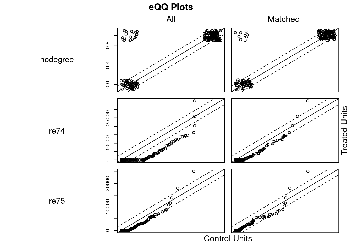
## Discarded 0 0plot(m.out1, type = "jitter", interactive = FALSE)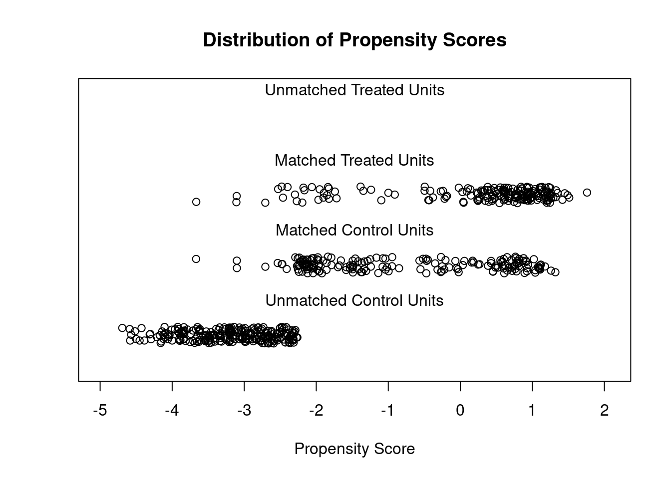
plot(summary(m.out1))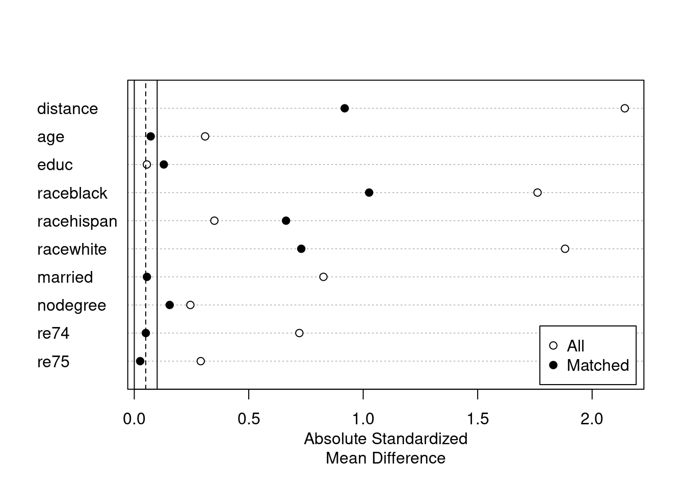
We see there are still some imbalance on variables such as “raceblack”. We can use more flexible models for the PS.
# GAM logistic PS with smoothing splines (s()):
m.out2 <- matchit(treat ~ s(age) + s(educ) +
                    race + married +
                    nodegree + re74 + re75,
                  data = lalonde,
                  distance = "gam")
summary(m.out2)
##
## Call:
## matchit(formula = treat ~ s(age) + s(educ) + race + married +
## nodegree + re74 + re75, data = lalonde, distance = "gam")
##
## Summary of Balance for All Data:
## Means Treated Means Control Std. Mean Diff. Var. Ratio eCDF Mean
## distance 0.6566 0.1481 1.9123 1.6161 0.4155
## raceblack 0.8432 0.2028 1.7615 . 0.6404
## racehispan 0.0595 0.1422 -0.3498 . 0.0827
## racewhite 0.0973 0.6550 -1.8819 . 0.5577
## married 0.1892 0.5128 -0.8263 . 0.3236
## nodegree 0.7081 0.5967 0.2450 . 0.1114
## re74 2095.5737 5619.2365 -0.7211 0.5181 0.2248
## re75 1532.0553 2466.4844 -0.2903 0.9563 0.1342
## age 25.8162 28.0303 -0.3094 0.4400 0.0813
## educ 10.3459 10.2354 0.0550 0.4959 0.0347
## eCDF Max
## distance 0.7172
## raceblack 0.6404
## racehispan 0.0827
## racewhite 0.5577
## married 0.3236
## nodegree 0.1114
## re74 0.4470
## re75 0.2876
## age 0.1577
## educ 0.1114
##
## Summary of Balance for Matched Data:
## Means Treated Means Control Std. Mean Diff. Var. Ratio eCDF Mean
## distance 0.6566 0.3055 1.3204 1.2324 0.1853
## raceblack 0.8432 0.4432 1.1002 . 0.4000
## racehispan 0.0595 0.1730 -0.4800 . 0.1135
## racewhite 0.0973 0.3838 -0.9667 . 0.2865
## married 0.1892 0.3568 -0.4278 . 0.1676
## nodegree 0.7081 0.6541 0.1189 . 0.0541
## re74 2095.5737 3521.7556 -0.2919 1.0512 0.1346
## re75 1532.0553 2056.2000 -0.1628 1.2120 0.0917
## age 25.8162 25.7081 0.0151 0.7958 0.0270
## educ 10.3459 10.1568 0.0941 0.6186 0.0270
## eCDF Max Std. Pair Dist.
## distance 0.5189 1.3204
## raceblack 0.4000 1.1002
## racehispan 0.1135 0.8914
## racewhite 0.2865 1.1491
## married 0.1676 1.0627
## nodegree 0.0541 0.9749
## re74 0.4270 0.8894
## re75 0.2378 0.8453
## age 0.0865 1.1619
## educ 0.0919 1.2447
##
## Sample Sizes:
## Control Treated
## All 429 185
## Matched 185 185
## Unmatched 244 0
## Discarded 0 0plot(m.out2, type = "jitter", interactive = FALSE)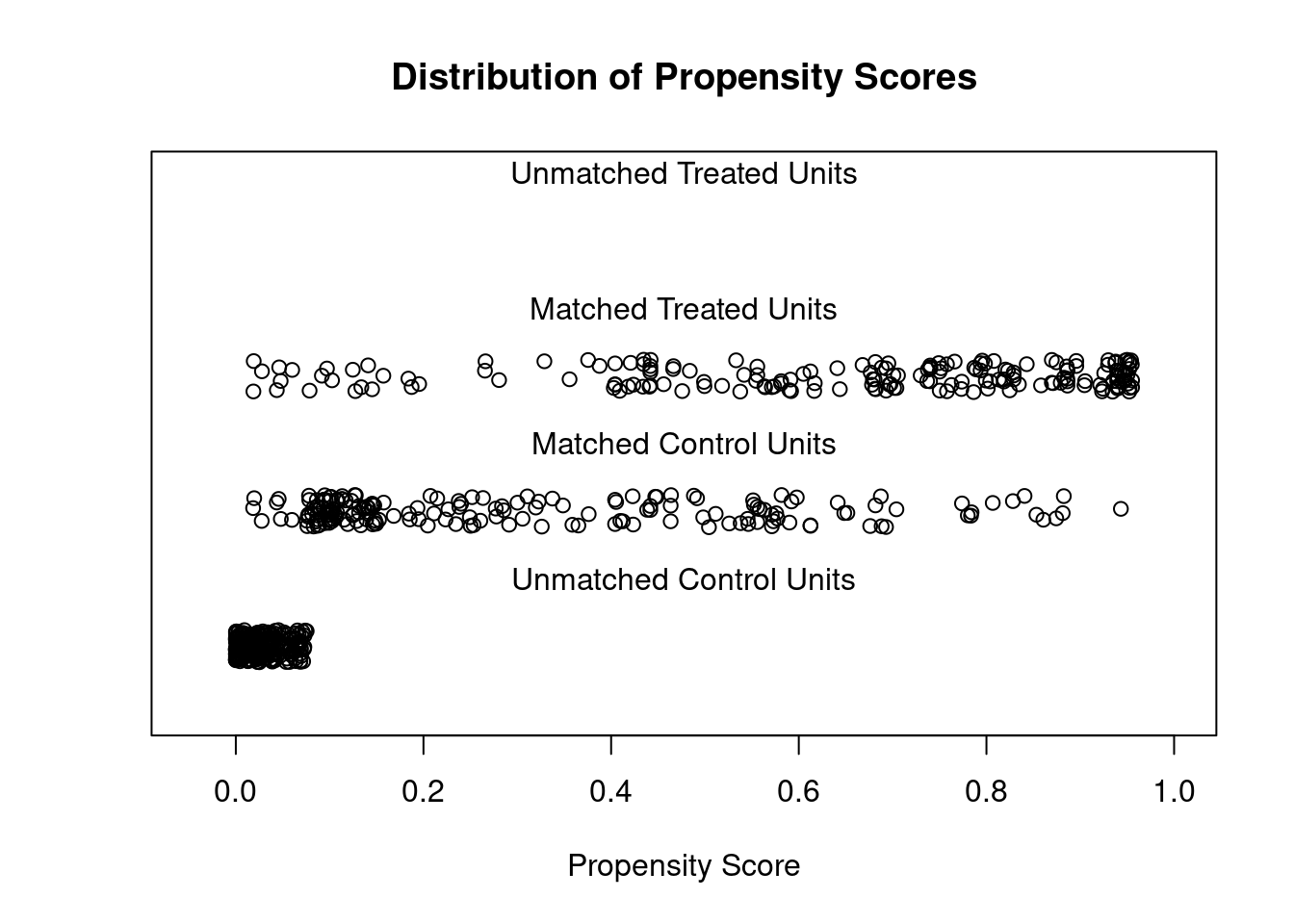
plot(summary(m.out2))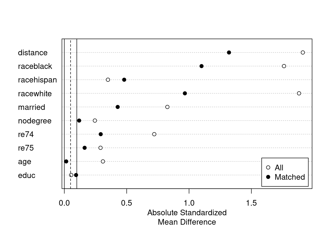
Or use CBPS.
# CBPS for ATC matching w/replacement, using the just-
# identified version of CBPS (setting method = "exact"):
m.out3 <- matchit(treat ~ age + educ + race + married +
                    nodegree + re74 + re75,
                  data = lalonde,
                  distance = "cbps",
                  estimand = "ATC",
                  distance.options = list(method = "exact"),
                  replace = TRUE)
summary(m.out3)
##
## Call:
## matchit(formula = treat ~ age + educ + race + married + nodegree +
## re74 + re75, data = lalonde, distance = "cbps", distance.options = list(method = "exact"),
## estimand = "ATC", replace = TRUE)
##
## Summary of Balance for All Data:
## Means Treated Means Control Std. Mean Diff. Var. Ratio eCDF Mean
## distance 0.2644 0.7687 -1.5395 0.9549 0.3515
## age 25.8162 28.0303 -0.2053 0.4400 0.0813
## educ 10.3459 10.2354 0.0387 0.4959 0.0347
## raceblack 0.8432 0.2028 1.5928 . 0.6404
## racehispan 0.0595 0.1422 -0.2369 . 0.0827
## racewhite 0.0973 0.6550 -1.1732 . 0.5577
## married 0.1892 0.5128 -0.6475 . 0.3236
## nodegree 0.7081 0.5967 0.2270 . 0.1114
## re74 2095.5737 5619.2365 -0.5190 0.5181 0.2248
## re75 1532.0553 2466.4844 -0.2838 0.9563 0.1342
## eCDF Max
## distance 0.5967
## age 0.1577
## educ 0.1114
## raceblack 0.6404
## racehispan 0.0827
## racewhite 0.5577
## married 0.3236
## nodegree 0.1114
## re74 0.4470
## re75 0.2876
##
## Summary of Balance for Matched Data:
## Means Treated Means Control Std. Mean Diff. Var. Ratio eCDF Mean
## distance 0.7649 0.7687 -0.0117 1.1610 0.0527
## age 27.5548 28.0303 -0.0441 0.4366 0.1098
## educ 11.0956 10.2354 0.3012 0.6742 0.0610
## raceblack 0.2914 0.2028 0.2203 . 0.0886
## racehispan 0.1259 0.1422 -0.0467 . 0.0163
## racewhite 0.5828 0.6550 -0.1520 . 0.0723
## married 0.5758 0.5128 0.1259 . 0.0629
## nodegree 0.4452 0.5967 -0.3089 . 0.1515
## re74 5490.4165 5619.2365 -0.0190 0.8172 0.1010
## re75 2022.3942 2466.4844 -0.1349 1.5681 0.0986
## eCDF Max Std. Pair Dist.
## distance 0.3636 0.0194
## age 0.2471 0.8657
## educ 0.2774 1.0115
## raceblack 0.0886 0.3131
## racehispan 0.0163 0.6474
## racewhite 0.0723 0.5345
## married 0.0629 0.6109
## nodegree 0.1515 1.0501
## re74 0.2494 0.7246
## re75 0.2774 1.0238
##
## Sample Sizes:
## Control Treated
## All 429 185.
## Matched (ESS) 429 6.57
## Matched 429 90.
## Unmatched 0 95.
## Discarded 0 0.plot(m.out3, type = "jitter", interactive = FALSE)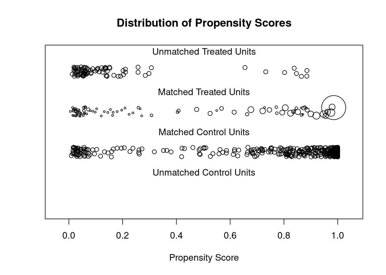
plot(summary(m.out3))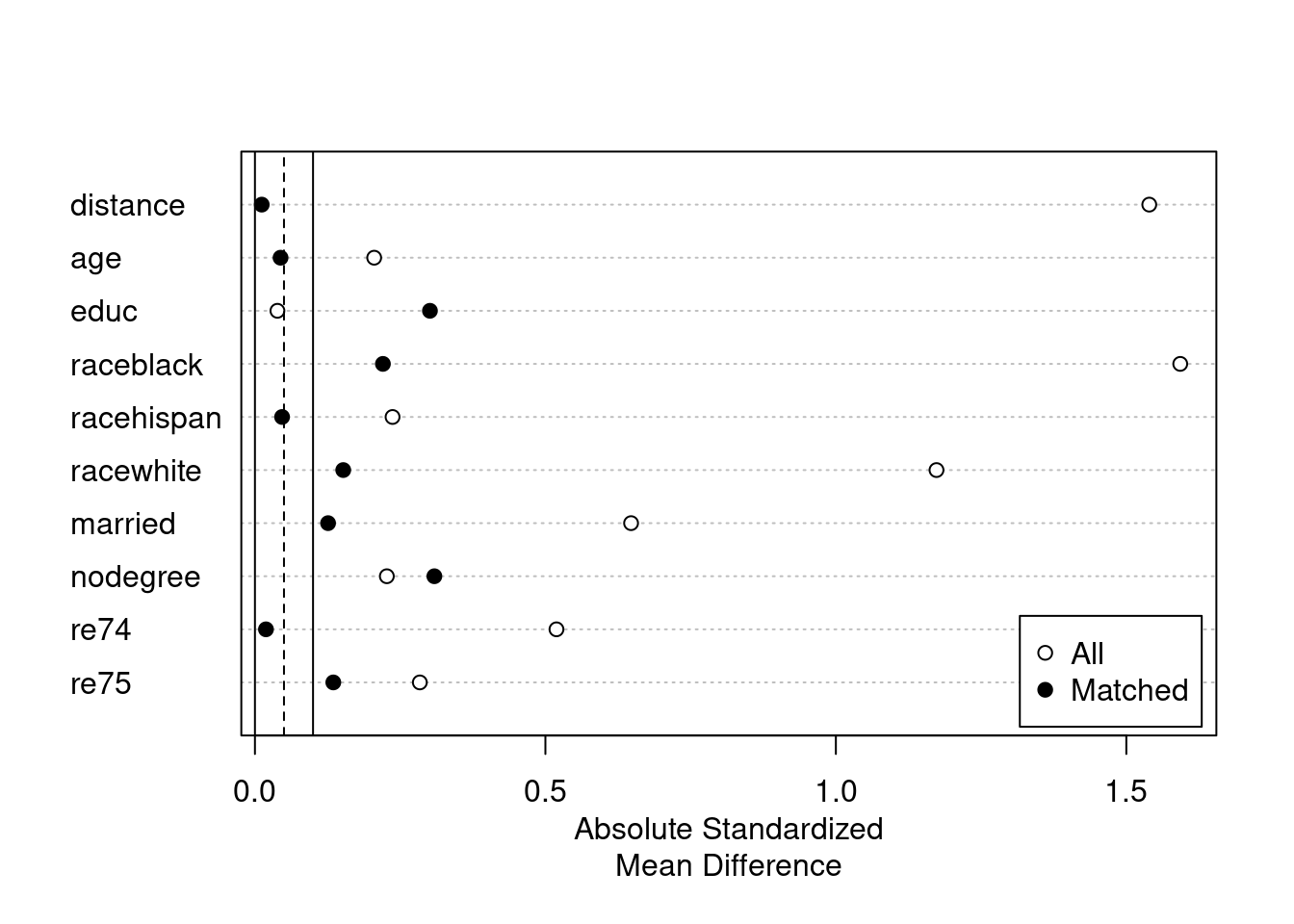
# Mahalanobis distance matching - no PS estimated
m.out4 <- matchit(treat ~ age + educ + race + married +
                    nodegree + re74 + re75,
                  data = lalonde,
                  distance = "mahalanobis")
summary(m.out4)
##
## Call:
## matchit(formula = treat ~ age + educ + race + married + nodegree +
## re74 + re75, data = lalonde, distance = "mahalanobis")
##
## Summary of Balance for All Data:
## Means Treated Means Control Std. Mean Diff. Var. Ratio eCDF Mean
## age 25.8162 28.0303 -0.3094 0.4400 0.0813
## educ 10.3459 10.2354 0.0550 0.4959 0.0347
## raceblack 0.8432 0.2028 1.7615 . 0.6404
## racehispan 0.0595 0.1422 -0.3498 . 0.0827
## racewhite 0.0973 0.6550 -1.8819 . 0.5577
## married 0.1892 0.5128 -0.8263 . 0.3236
## nodegree 0.7081 0.5967 0.2450 . 0.1114
## re74 2095.5737 5619.2365 -0.7211 0.5181 0.2248
## re75 1532.0553 2466.4844 -0.2903 0.9563 0.1342
## eCDF Max
## age 0.1577
## educ 0.1114
## raceblack 0.6404
## racehispan 0.0827
## racewhite 0.5577
## married 0.3236
## nodegree 0.1114
## re74 0.4470
## re75 0.2876
##
## Summary of Balance for Matched Data:
## Means Treated Means Control Std. Mean Diff. Var. Ratio eCDF Mean
## age 25.8162 24.9081 0.1269 0.5327 0.0695
## educ 10.3459 10.4324 -0.0430 0.8345 0.0108
## raceblack 0.8432 0.4649 1.0407 . 0.3784
## racehispan 0.0595 0.0595 0.0000 . 0.0000
## racewhite 0.0973 0.4757 -1.2767 . 0.3784
## married 0.1892 0.2486 -0.1518 . 0.0595
## nodegree 0.7081 0.6595 0.1070 . 0.0486
## re74 2095.5737 3305.4420 -0.2476 0.8705 0.1012
## re75 1532.0553 1957.5097 -0.1322 1.0071 0.0654
## eCDF Max Std. Pair Dist.
## age 0.2378 0.6195
## educ 0.0486 0.2903
## raceblack 0.3784 1.0407
## racehispan 0.0000 0.0000
## racewhite 0.3784 1.2767
## married 0.0595 0.1794
## nodegree 0.0486 0.1070
## re74 0.3351 0.4546
## re75 0.2162 0.4113
##
## Sample Sizes:
## Control Treated
## All 429 185
## Matched 185 185
## Unmatched 244 0
## Discarded 0 0m.out4$distance #NULL## NULLplot(m.out4, interactive = FALSE)
plot(summary(m.out4))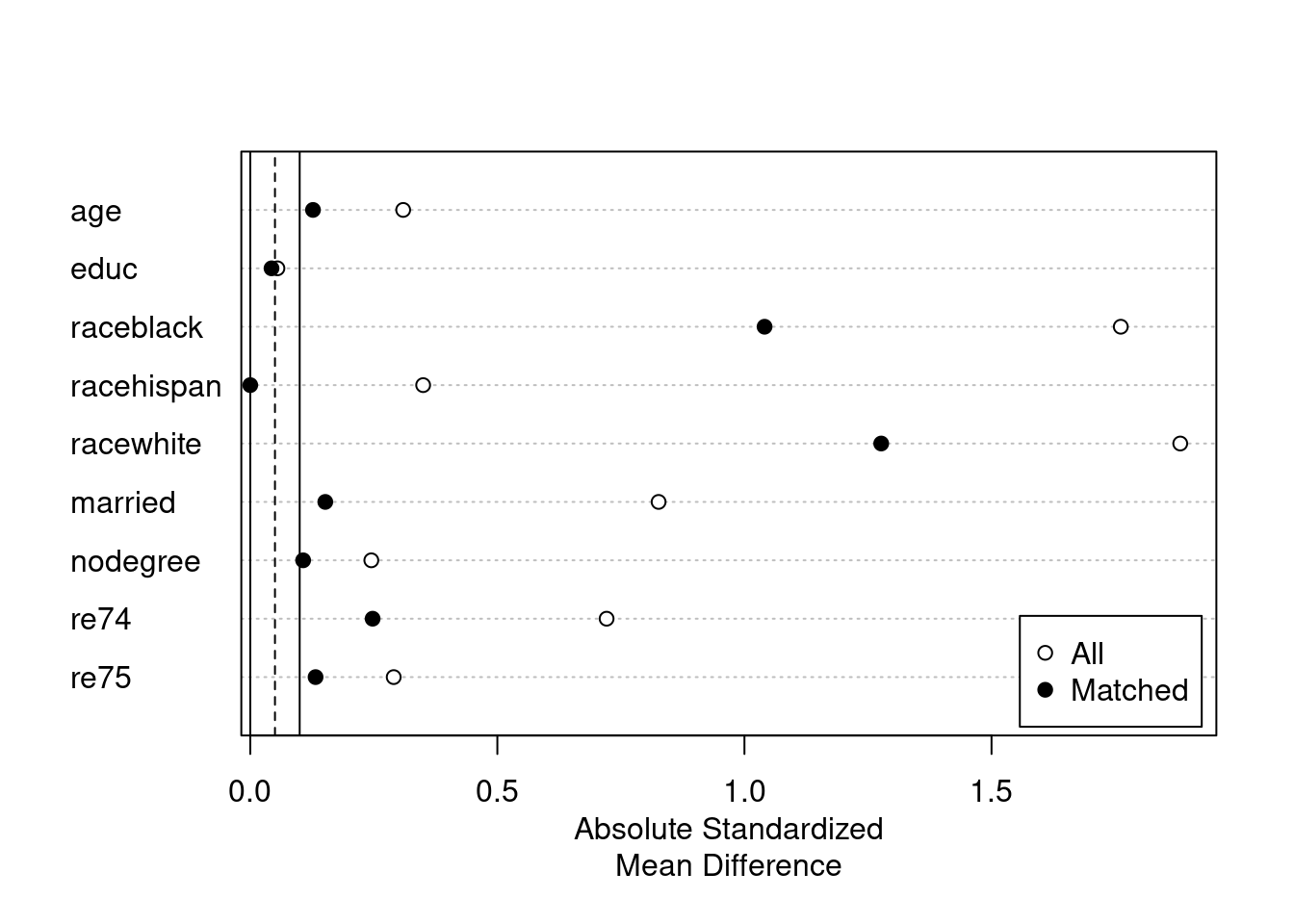
# Full matching on a probit PS
m.out5 <- matchit(treat ~ age + educ + race + married +
                    nodegree + re74 + re75,
                  data = lalonde,
                  method = "full",
                  distance = "glm",
                  link = "probit")

summary(m.out5)
##
## Call:
## matchit(formula = treat ~ age + educ + race + married + nodegree +
## re74 + re75, data = lalonde, method = "full", distance = "glm",
## link = "probit")
##
## Summary of Balance for All Data:
## Means Treated Means Control Std. Mean Diff. Var. Ratio eCDF Mean
## distance 0.5773 0.1817 1.8276 0.8777 0.3774
## age 25.8162 28.0303 -0.3094 0.4400 0.0813
## educ 10.3459 10.2354 0.0550 0.4959 0.0347
## raceblack 0.8432 0.2028 1.7615 . 0.6404
## racehispan 0.0595 0.1422 -0.3498 . 0.0827
## racewhite 0.0973 0.6550 -1.8819 . 0.5577
## married 0.1892 0.5128 -0.8263 . 0.3236
## nodegree 0.7081 0.5967 0.2450 . 0.1114
## re74 2095.5737 5619.2365 -0.7211 0.5181 0.2248
## re75 1532.0553 2466.4844 -0.2903 0.9563 0.1342
## eCDF Max
## distance 0.6413
## age 0.1577
## educ 0.1114
## raceblack 0.6404
## racehispan 0.0827
## racewhite 0.5577
## married 0.3236
## nodegree 0.1114
## re74 0.4470
## re75 0.2876
##
## Summary of Balance for Matched Data:
## Means Treated Means Control Std. Mean Diff. Var. Ratio eCDF Mean
## distance 0.5773 0.5764 0.0045 0.9949 0.0043
## age 25.8162 25.5347 0.0393 0.4790 0.0787
## educ 10.3459 10.5381 -0.0956 0.6192 0.0253
## raceblack 0.8432 0.8389 0.0119 . 0.0043
## racehispan 0.0595 0.0492 0.0435 . 0.0103
## racewhite 0.0973 0.1119 -0.0493 . 0.0146
## married 0.1892 0.1633 0.0660 . 0.0259
## nodegree 0.7081 0.6577 0.1110 . 0.0504
## re74 2095.5737 2100.2150 -0.0009 1.3467 0.0314
## re75 1532.0553 1561.4420 -0.0091 1.5906 0.0536
## eCDF Max Std. Pair Dist.
## distance 0.0486 0.0198
## age 0.2742 1.2843
## educ 0.0730 1.2179
## raceblack 0.0043 0.0162
## racehispan 0.0103 0.4412
## racewhite 0.0146 0.3454
## married 0.0259 0.4473
## nodegree 0.0504 0.9872
## re74 0.1881 0.8387
## re75 0.1984 0.8240
##
## Sample Sizes:
## Control Treated
## All 429. 185
## Matched (ESS) 50.76 185
## Matched 429. 185
## Unmatched 0. 0
## Discarded 0. 0plot(m.out5, type = "jitter", interactive = FALSE)
plot(summary(m.out5))
Estimation
After we get a matched data that we think is good enough, we can estimate the treatment effect.
m.data <- match_data(m.out5)

head(m.data)
## treat age educ race married nodegree re74 re75 re78 distance
## NSW1 1 37 11 black 1 1 0 0 9930.0460 0.6356769
## NSW2 1 22 9 hispan 0 1 0 0 3595.8940 0.2298151
## NSW3 1 30 12 black 0 0 0 0 24909.4500 0.6813558
## NSW4 1 27 11 black 0 1 0 0 7506.1460 0.7690590
## NSW5 1 33 8 black 0 1 0 0 289.7899 0.6954138
## NSW6 1 22 9 black 0 1 0 0 4056.4940 0.6943658
## weights subclass
## NSW1 1 1
## NSW2 1 55
## NSW3 1 63
## NSW4 1 70
## NSW5 1 79
## NSW6 1 86What “match_data” does is to grab the matched data with a few additional variables such as “weights”, “subclass”, and “distance”. Then we can use it in a simple linear model with weights.
library("marginaleffects")

fit <- lm(re78 ~ treat * (age + educ + race + married +
                            nodegree + re74 + re75),
          data = m.data,
          weights = weights)

avg_comparisons(fit,
                variables = "treat",
                vcov = ~subclass,
                newdata = subset(treat == 1))
##
## Estimate Std. Error z Pr(>|z|) S 2.5 % 97.5 %
## 1977 704 2.81 0.00501 7.6 596 3357
##
## Term: treat
## Type: response
## Comparison: 1 - 0Note we allow interaction of treatment and covariates, but we do no need to demean the covariates here, since we are relying on “marginaleffects” and its “avg_comparisons” function to compute the average treatment effect. The “newdata” argument is used to specify the effect, in this case ATT. Note the weights are generated this way: since it’s ATT, all treated units are weighted by 1, and control units are weighted by \(p/(1-p)\), where \(p\) is proportion of treated units in the subclass. Anyway, for full matching, we get the comparison of potential outcomes for the treated, with weights, and clustered standard errors on subclasses, because that the level the comparison is conducted.