Why DDDiD

Guido Imbens has been saying DDDiD (Don’t Do Diff in Diff). But why?

To see that, DiD objective function (in the form of TWFE) is:

\[ \small (\hat \tau^{did}, \hat \mu, \hat \alpha, \hat \beta) = \underset{\tau, \mu, \alpha, \beta}{argmin} { \Sigma_{i=1}^N \Sigma_{t=1}^T (Y_{it} - \mu - \alpha_i - \beta_t - W_{it} \tau)^2}\]

We can see that in this objective function, we are allowing only \(\alpha_i\) and \(\beta_t\) to capture the difference between units and time periods. The obvious drawback is that control units that are less similar to a treated unit is given the same weight as those that are more similar. A time peiod that is far from the beginning of the treatment period is given the same weight as those that are closer. Say the treatment period is 2000, we have observations from 1988 to 2005, then 1988 observations are the same as 1999 observations. This is not ideal. The same logic applies to the units.

Synthetic Control

SC objective function: \[ (\hat \tau^{sc}, \hat \mu, \hat \beta) = \underset{\tau, \mu, \beta}{argmin} { \Sigma_{i=1}^N \Sigma_{t=1}^T (Y_{it} - \mu - \beta_t - W_{it} \tau)^2 \hat \omega^{sc}}\]

It’s a weighted version of DiD. In this sense, DiD is a special case of SC, setting all weights to 1. The weights are set to optimally match donor units to treated unit so that they are as close as possible, in each time point. Note there is no \(\alpha_i\), since it’s forced to be 0. However, there is no time weight.

Synthetic DiD

Arkhangelsky et al (2021) tries to combine the idea of DiD and SC. SC assigns different weights to different control units. The standard DiD is a TWFE, assigning equal weights to all time periods and units.

\[ \small (\hat \tau^{sdid}, \hat \mu, \hat \alpha, \hat \beta) = \underset{\tau, \mu, \alpha, \beta}{argmin} { \Sigma_{i=1}^N \Sigma_{t=1}^T (Y_{it} - \mu - \alpha_i - \beta_t - W_{it} \tau)^2} \hat \omega_i^{sdid} \lambda_t^{sdid}\]

SDiD sets another weight in addition to SC weights, which changes over time. The SC weights are trying to construct a control unit that is close to the treated unit; the SDiD weights are trying to put more weights on pre-treatment periods that are more similar to post-treatment periods.

Example from synthdid

library(synthdid)
data('california_prop99')
setup = panel.matrices(california_prop99)
tau.hat = synthdid_estimate(setup$Y, setup$N0, setup$T0)
summary(tau.hat)

## $estimate
## [1] -15.60383
## 
## $se
##      [,1]
## [1,]   NA
## 
## $controls
##                estimate 1
## Nevada              0.124
## New Hampshire       0.105
## Connecticut         0.078
## Delaware            0.070
## Colorado            0.058
## Illinois            0.053
## Nebraska            0.048
## Montana             0.045
## Utah                0.042
## New Mexico          0.041
## Minnesota           0.039
## Wisconsin           0.037
## West Virginia       0.034
## North Carolina      0.033
## Idaho               0.031
## Ohio                0.031
## Maine               0.028
## Iowa                0.026
## 
## $periods
##      estimate 1
## 1988      0.427
## 1986      0.366
## 1987      0.206
## 
## $dimensions
##           N1           N0 N0.effective           T1           T0 T0.effective 
##        1.000       38.000       16.388       12.000       19.000        2.783

tau.sc   = sc_estimate(setup$Y, setup$N0, setup$T0)
tau.did  = did_estimate(setup$Y, setup$N0, setup$T0)
estimates = list(tau.did, tau.sc, tau.hat)
names(estimates) = c('Diff-in-Diff', 'Synthetic Control', 'Synthetic Diff-in-Diff')
print(unlist(estimates))

##           Diff-in-Diff      Synthetic Control Synthetic Diff-in-Diff 
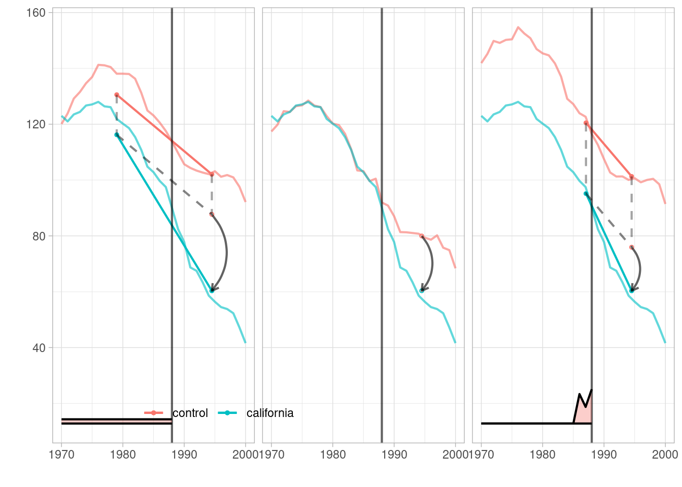
##              -27.34911              -19.61966              -15.60383

plot <- synthdid_plot(estimates, facet.vertical=FALSE,
              control.name='control', treated.name='california',
              lambda.comparable=TRUE, se.method = 'none',
              trajectory.linetype = 1, line.width=.75, effect.curvature=-.4,
              trajectory.alpha=.7, effect.alpha=.7,
              diagram.alpha=1, onset.alpha=.7) +
    theme(legend.position=c(.26,.07), legend.direction='horizontal',
          legend.key=element_blank(), legend.background=element_blank(),
          strip.background=element_blank(), strip.text.x = element_blank())
plot

Note: \(\lambda_t\) is plotted at the bottom.

Summary

To me, “DDDiD” is saying DiD is too simple. Even if all the identification assumptions are correct for DiD, namely parallel trend and no anticipation, there are still better ways to do it, in the sense of putting weights on units and time periods, such as synthetic DiD.