The problem
g-estimation is a method to estimate the causal effect of a time varying treatment or covariates. The method is developed by Robins (1986) and Robins and Rotnitzky (1992). The method is also known as the g-methods.
We can imagine such a scenario. Suppose \(A0\) and \(A1\) are time 0 and time 1 treatment, can be binary or continuous. \(L1\) is a time 1 covariate. It can be some intermediate outcome. Say HbA1c. HbA1c can be a result of treatment \(A0\). Then it can be a cause for the next period treatment \(A1\). \(Y\) is the outcome. \(U\) is the unmeasured confounder. The causal diagram is shown below. How do we estimate the effect of treatment?
library(dagitty)
library(ggdag)
library(ggplot2)
library(gfoRmula)
library(gmethods)
library(tidyverse)

dag <- dagify(
  Y ~ A1 + A0 + L1 ,
  A1 ~ A0 + L1,
  L1 ~ A0 ,
  coords = time_ordered_coords()
)

dag %>%
  ggplot(aes(x = x, y = y, xend = xend, yend = yend)) +
  geom_dag_point() +
  geom_dag_edges_arc() +
  geom_dag_text() +
  theme_dag()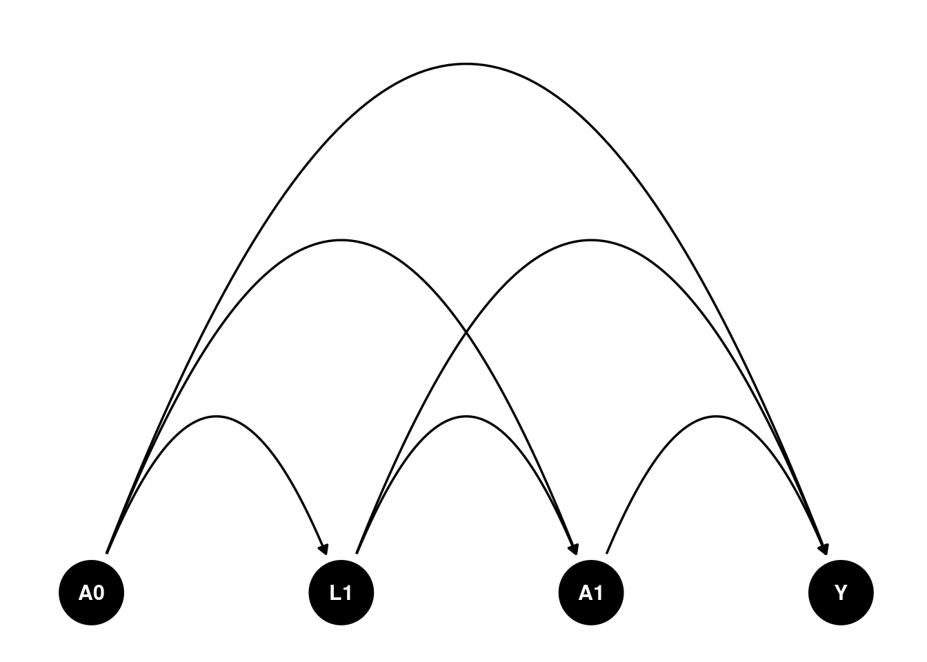
Assumptions
There are four potential outcomes, with \(A_0\) and \(A_1\) can be 0 or 1. The causal estimand is \[ \tau_{a_o,a_1,a_o',a_1'} = E[Y^{a_0,a_1} - Y^{a_0',a_1'}]\]
To idenfity the effects, we need assumptions.
- Sequential ignorability \[ Y^{a_0,a_1} \perp A_0\] \[ Y^{a_0,a_1} \perp A_1^{a_0} | A_0, L_1^{a_0}\]
In general, treatment at time t is randomized with probabilities depending on the observed past, including covariates, intermediate outcomes, that is, at any time t \[ Y^{\bar a}_t ⊥ A_t | H_t \] where \({\bar a}_t = (a_1, ..., a_t)\), and \(H_t\) is the history of treatment and covariates up to time t \[H_t=(A_0, A_1, ..., A_{t-1}; L_1,..., L_{t-1})\].
- Positivity
\[ 0 < P(A_0=1) < 1\] \[ 0 < P(A_1=1|A_0=1, L_1) < 1\]
In general, \[ 0 < P(A_t=1|H_t) < 1\]
- Consistency
\[ Y^{a_0,a_1} = Y | (A_0=a_0,A_1=a_1)\]
Identifiability
\[ \begin{align} E[Y^{a_0,a_1} &= E[Y^{a_0,a_1} | A_0=a_0] \\ &= E[Y^{A_0,a_1} | A_0=a_0] \\ &= \sum_{l=0,1}E[Y^{A_0,a_1} | A_0=a_0, L=l] P(L=l | A_0=a_0) \\ &= \sum_{l=0,1}E[Y^{A_0,a_1} | A_0=a_0, L=l, A_1=a_1] P(L=l | A_0=a_0) \\ &= \sum_{l=0,1}E[Y^{A_0,A_1} | A_0=a_0, L=l, A_1=a_1] P(L=l | A_0=a_0) \end{align} \]
This can be expanded to the general case. Basically start from the first period, then the second, based on the first, and so on.
Estimation
There are two types of componenets in the g-estimation. The first is the outcome model, then there are models for time-varying covariates, or intermediate outcomes (confounders).
Parametric g-formula
In this simple case, if \(Y\) is continuous, we can use a linear model. If \(Y\) is binary, we can use a logistic model.
\[ E[Y | A_0, A_1, L_1] = \beta_0 + \beta_1 A_0 + \beta_2 L_1 + \beta_3 A_1\]
Suppose \(L_1\) is binary,
\[P(L_1=1 | A_0) = logit^{-1}(\gamma_0 + \gamma_1 A_0)\] \[ L_1 | A_0 \sim Bernoulli(\gamma_0 + \gamma_1 A_0)\]
We may need to simulate the distribution of the time-varying covariates for the expected value of the potential outcomes.
an example
I am following Christopher Boyer’s example in his teaching page: https://christopherbboyer.com/about.
The first example is from his lab3 teaching page.
First we set up a simulated data set.
# setting up the data -----------------------------------------------------

# The code below creates the frequency table, and then turns it into long format
# data. Read through the code carefully and run it.

# re-create the frequency table for homework 3
hw3_freq <- tribble(
  ~A_0, ~L_1, ~A_1, ~N, ~Y_1,
  0, 0, 0, 6000, 60,
  0, 0, 1, 2000, 60,
  0, 1, 0, 2000, 210,
  0, 1, 1, 6000, 210,
  1, 0, 0, 3000, 240,
  1, 0, 1, 1000, 240,
  1, 1, 0, 3000, 120,
  1, 1, 1, 9000, 120
)

# expand the frequency table to 1 row per person
# (first just assign everyone the average Y value)
dat <- uncount(hw3_freq, N) %>%
  # give those rows an id number
  rowid_to_column(var = "id") %>%
  # for each of the variables except for id, split it into two
  # rows, one for each time point
  pivot_longer(-id,
               names_to = c(".value", "time"),
               names_sep = "_"
  ) %>%
  # make sure that time is read as a number
  mutate(time = parse_number(time),
         # add some random error to Y
         # (nrow(.) means a different value for each row of the dataset in use
         Y = Y + rnorm(nrow(.), 0, 10))


# create lagged variables
t1 <- dat %>%
  mutate(lag_A = lag(A)) %>%
  filter(time == 1)
Then calculate the g-formula by hand.
First for \(E[Y^{1,1}]\).
# fit models for covariate and outcome given past on t1
L_mod <- glm(L ~ lag_A, data = t1, family = binomial())
Y_mod <- glm(Y ~ A * lag_A * L, data = t1)

# create new data set with space for 10,000 simulated entries
nsim <- 10000
baseline_pop <- tibble(id = 1:nsim)

# fix intervention values in the new data set to be consistent with the regime
new_dat_11 <- baseline_pop %>%
  mutate(lag_A = 1, A = 1)

# predict covariate means at time 1
new_dat_11$pL <- predict(L_mod, newdata = new_dat_11, type = "response")

# simulate covariate values at time 1
new_dat_11$L <- rbinom(nsim, 1, new_dat_11$pL)

# predict outcome at time 1 based on simulated covariates and fixed treatments
new_dat_11$Ey <- predict(Y_mod, newdata = new_dat_11, type = "response")

# take mean across all simulations to get g-formula estimate!
mean(new_dat_11$Ey)
## [1] 150.657Then for \(E[Y^{0,0}]\).
# for 0, 0
new_dat_00 <- baseline_pop %>%
  mutate(lag_A = 0, A = 0)

# predict covariate means at time 1
new_dat_00$pL <- predict(L_mod, newdata = new_dat_00, type = "response")

# simulate covariate values at time 1
new_dat_00$L <- rbinom(nsim, 1, new_dat_00$pL)

# predict outcome at time 1 based on simulated covariates and fixed treatments
new_dat_00$Ey <- predict(Y_mod, newdata = new_dat_00, type = "response")

# take mean across all simulations to get g-formula estimate!
mean(new_dat_00$Ey)
## [1] 134.6698Now with the gfoRmula package.
# running the g-formula ---------------------------------------------------

# add your comments to the lines below
id <- "id"
time_name <- "time"
covnames <- c("L", "A")
outcome_name <- "Y"
#
outcome_type <- "continuous_eof"
#
histories <- c(lagged)
#
histvars <- list(c("A"))
#
covtypes <- c("binary", "binary")
covparams <- list(covmodels = c(
  L ~ lag1_A,
  A ~ lag1_A * L
))
ymodel <- Y ~ A * L * lag1_A
#
intvars <- list("A", "A", "A", "A")
#
interventions <- list(
  list(c(static, c(0, 0))),
  list(c(static, c(0, 1))),
  list(c(static, c(1, 0))),
  list(c(static, c(1, 1)))
)
int_descript <- c(
  "0, 0",
  "0, 1",
  "1, 0",
  "1, 1"
)

# put it all together
# (the warning "obs_data was coerced to a data table" is fine!)
gform_res <- gfoRmula::gformula(
  obs_data = dat,
  id = id,
  time_name = time_name,
  covnames = covnames,
  outcome_name = outcome_name,
  outcome_type = outcome_type,
  covtypes = covtypes,
  covparams = covparams,
  ymodel = ymodel,
  intvars = intvars,
  interventions = interventions,
  int_descript = int_descript,
  ref_int = 1,
  histories = histories,
  histvars = histvars,
  sim_data_b = TRUE,
  seed = 345636
)
# Use the following code to explore the results. (You can ignore Intervention 0,
# the natural course intervention, for now.) How many models were fit? How can
# you tell which of the data in the `sim_data` object was simulated or predicted
# from a model? Does these results match your answers to the earlier questions,
gform_res
## PREDICTED RISK UNDER MULTIPLE INTERVENTIONS
##
## Intervention Description
## 0 Natural course
## 1 0, 0
## 2 0, 1
## 3 1, 0
## 4 1, 1
##
## Sample size = 32000, Monte Carlo sample size = 32000
## Number of bootstrap samples = 0
## Reference intervention = 1
##
##
##
## k Interv. NP mean g-form mean Mean ratio Mean difference % Intervened On
## <num> <num> <num> <num> <num> <num> <num>
## 1 0 142.4411 143.0339 1.057266 7.747306 0.00000
## 1 1 NA 135.2866 1.000000 0.000000 75.12188
## 1 2 NA 135.5298 1.001798 0.243191 74.87812
## 1 3 NA 150.0048 1.108793 14.718196 80.85625
## 1 4 NA 150.0192 1.108899 14.732548 69.14375
## Aver % Intervened On
## <num>
## 0.00000
## 50.25469
## 49.74531
## 55.99375
## 44.00625gform_res$coeffs## $L
## (Intercept) lag1_A
## -5.868391e-14 1.098612e+00
##
## $A
## (Intercept) lag1_A L lag1_A:L
## -1.098612e+00 -6.322990e-13 2.197225e+00 2.925534e-13
##
## $Y
## (Intercept) A L lag1_A A:L
## 59.81251171 0.36039695 150.22527728 180.09937469 -0.23328912
## A:lag1_A L:lag1_A A:L:lag1_A
## -0.11174272 -270.26140641 -0.07953104gform_res$sim_data## $`Natural course`
## id time L A eligible_pt intervened lag1_A Ey
## <int> <num> <num> <num> <lgcl> <num> <num> <num>
## 1: 1 0 NA 0 TRUE 0 0 NA
## 2: 1 1 0 0 TRUE 0 0 59.81251
## 3: 2 0 NA 0 TRUE 0 0 NA
## 4: 2 1 0 0 TRUE 0 0 59.81251
## 5: 3 0 NA 0 TRUE 0 0 NA
## ---
## 63996: 31998 1 1 1 TRUE 0 1 119.81159
## 63997: 31999 0 NA 1 TRUE 0 0 NA
## 63998: 31999 1 1 1 TRUE 0 1 119.81159
## 63999: 32000 0 NA 1 TRUE 0 0 NA
## 64000: 32000 1 1 1 TRUE 0 1 119.81159
##
## $`0, 0`
## id time L A eligible_pt intervened lag1_A Ey
## <int> <num> <num> <num> <lgcl> <lgcl> <num> <num>
## 1: 1 0 NA 0 TRUE FALSE 0 NA
## 2: 1 1 0 0 TRUE FALSE 0 59.81251
## 3: 2 0 NA 0 TRUE FALSE 0 NA
## 4: 2 1 0 0 TRUE FALSE 0 59.81251
## 5: 3 0 NA 0 TRUE FALSE 0 NA
## ---
## 63996: 31998 1 1 0 TRUE TRUE 0 210.03779
## 63997: 31999 0 NA 0 TRUE TRUE 0 NA
## 63998: 31999 1 1 0 TRUE TRUE 0 210.03779
## 63999: 32000 0 NA 0 TRUE TRUE 0 NA
## 64000: 32000 1 0 0 TRUE FALSE 0 59.81251
##
## $`0, 1`
## id time L A eligible_pt intervened lag1_A Ey
## <int> <num> <num> <num> <lgcl> <lgcl> <num> <num>
## 1: 1 0 NA 0 TRUE FALSE 0 NA
## 2: 1 1 0 1 TRUE TRUE 0 60.17291
## 3: 2 0 NA 0 TRUE FALSE 0 NA
## 4: 2 1 0 1 TRUE TRUE 0 60.17291
## 5: 3 0 NA 0 TRUE FALSE 0 NA
## ---
## 63996: 31998 1 1 1 TRUE FALSE 0 210.16490
## 63997: 31999 0 NA 0 TRUE TRUE 0 NA
## 63998: 31999 1 1 1 TRUE FALSE 0 210.16490
## 63999: 32000 0 NA 0 TRUE TRUE 0 NA
## 64000: 32000 1 0 1 TRUE TRUE 0 60.17291
##
## $`1, 0`
## id time L A eligible_pt intervened lag1_A Ey
## <int> <num> <num> <num> <lgcl> <lgcl> <num> <num>
## 1: 1 0 NA 1 TRUE TRUE 0 NA
## 2: 1 1 1 0 TRUE TRUE 1 119.8758
## 3: 2 0 NA 1 TRUE TRUE 0 NA
## 4: 2 1 1 0 TRUE TRUE 1 119.8758
## 5: 3 0 NA 1 TRUE TRUE 0 NA
## ---
## 63996: 31998 1 1 0 TRUE TRUE 1 119.8758
## 63997: 31999 0 NA 1 TRUE FALSE 0 NA
## 63998: 31999 1 1 0 TRUE TRUE 1 119.8758
## 63999: 32000 0 NA 1 TRUE FALSE 0 NA
## 64000: 32000 1 1 0 TRUE TRUE 1 119.8758
##
## $`1, 1`
## id time L A eligible_pt intervened lag1_A Ey
## <int> <num> <num> <num> <lgcl> <lgcl> <num> <num>
## 1: 1 0 NA 1 TRUE TRUE 0 NA
## 2: 1 1 1 1 TRUE FALSE 1 119.8116
## 3: 2 0 NA 1 TRUE TRUE 0 NA
## 4: 2 1 1 1 TRUE FALSE 1 119.8116
## 5: 3 0 NA 1 TRUE TRUE 0 NA
## ---
## 63996: 31998 1 1 1 TRUE FALSE 1 119.8116
## 63997: 31999 0 NA 1 TRUE FALSE 0 NA
## 63998: 31999 1 1 1 TRUE FALSE 1 119.8116
## 63999: 32000 0 NA 1 TRUE FALSE 0 NA
## 64000: 32000 1 1 1 TRUE FALSE 1 119.8116A second example
Chistopher Boyer has a package “gmethods” that can be used to estimate the g-formula. To me it’s a bit more intuitive than the gfoRmula package. Here is an example in the “gmethods” package, with the same model in the “gfoRmula” package.
The example dataset continuous_eofdata again consists of 7,500 observations on 2,500 individuals with a maximum of 7 follow-up times, where the outcome corresponds to a characteristic only in the last interval (e.g., systolic blood pressure in interval 7). The variables in the dataset are: t0: The time index id: A unique identifier for each individual L1: A time-varying covariate; categorical L2: A time-varying covariate; continuous L3: A baseline covariate; continuous A: The treatment variable; binary Y: The outcome of interest; continuous
The goal is to estimate the mean outcome at time \(K + 1 = 7\) under ‘‘never treat’’ versus ‘‘always treat.’’
The DAG would be something like:
dag <- dagify(
  Y ~ A + L1 + L2 + L3 + lag1_A + lag1_L1 + lag1_L2 ,
  L1 ~ lag1_A + lag1_L1 + lag1_L2 + L3 ,
  L2 ~ lag1_A + L1 + lag1_L1 + lag1_L2 + L3,
  A ~ lag1_A + L1 + L2 + lag1_L1 + lag1_L2 + L3,
  coords = time_ordered_coords()
)

dag %>%
  ggplot(aes(x = x, y = y, xend = xend, yend = yend)) +
  geom_dag_point() +
  geom_dag_edges_arc() +
  geom_dag_text() +
  theme_dag()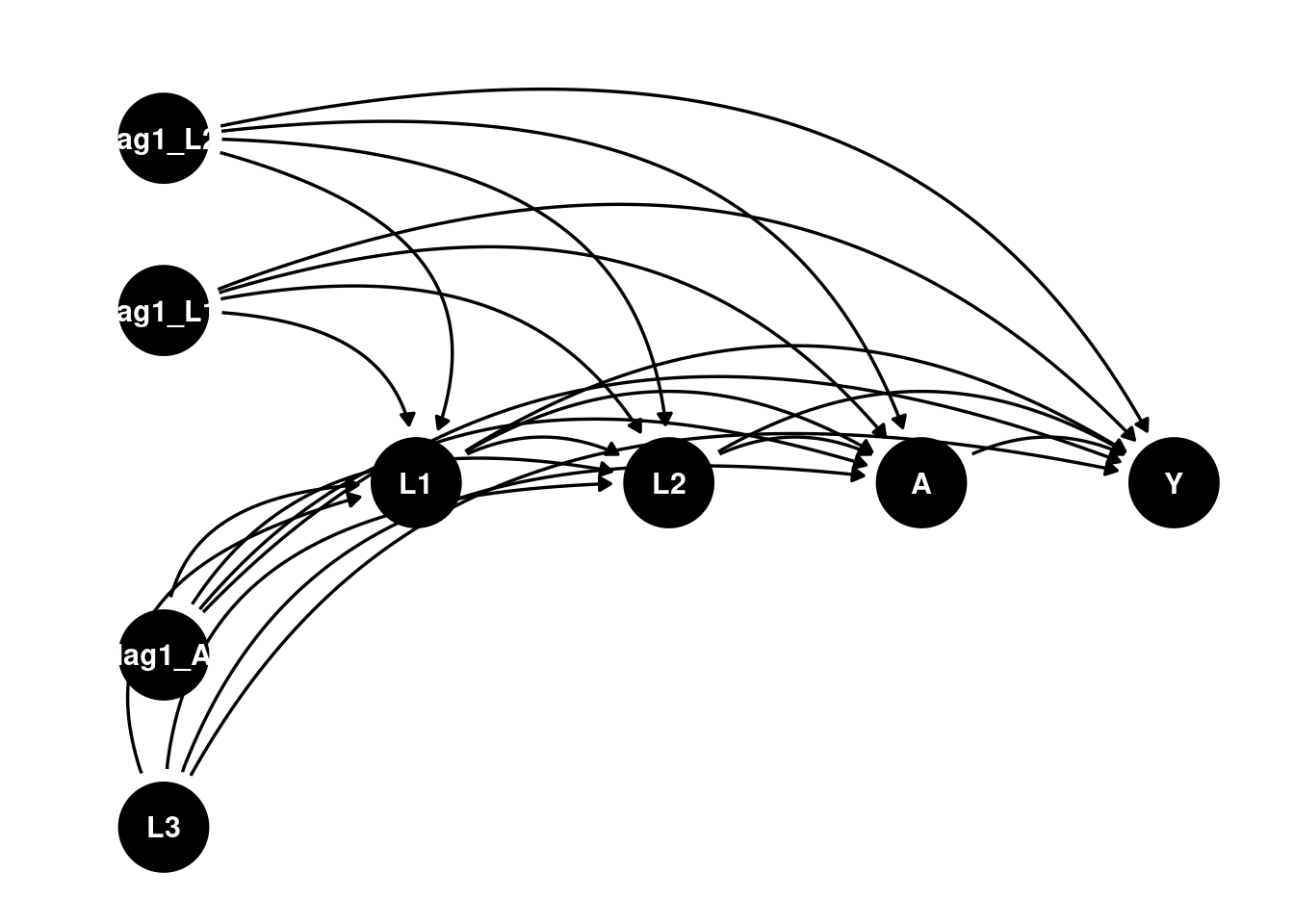
gFormula results
First use the gFormula package.
id <- 'id'
time_name <- 't0'
covnames <- c('L1', 'L2', 'A')
outcome_name <- 'Y'
covtypes <- c('categorical', 'normal', 'binary')
histories <- c(lagged)
histvars <- list(c('A', 'L1', 'L2'))
covparams <- list(covmodels = c(L1 ~ lag1_A + lag1_L1 + L3 + t0 +
                                 lag1_L2,
                                L2 ~ lag1_A + L1 + lag1_L1 + lag1_L2 + L3 + t0,
                                A ~ lag1_A + L1 + L2 + lag1_L1 + lag1_L2 + L3 + t0))
ymodel <- Y ~ A + L1 + L2 + lag1_A + lag1_L1 + lag1_L2 + L3
intvars <- list('A', 'A')
interventions <- list(list(c(static, rep(0, 7))),
                      list(c(static, rep(1, 7))))
int_descript <- c('Never treat', 'Always treat')
nsimul <- 50000

gform_cont_eof <- gformula_continuous_eof(obs_data = continuous_eofdata,
                                          id = id,
                                          time_name = time_name,
                                          covnames = covnames,
                                          outcome_name = outcome_name,
                                          covtypes = covtypes,
                                          covparams = covparams, ymodel = ymodel,
                                          intvars = intvars,
                                          interventions = interventions,
                                          int_descript = int_descript,
                                          histories = histories,
                                          histvars = histvars,
                                          model_fits = TRUE,
                                          basecovs = c("L3"),
                                          nsimul = nsimul, seed = 1234)
gform_cont_eof
## PREDICTED RISK UNDER MULTIPLE INTERVENTIONS
##
## Intervention Description
## 0 Natural course
## 1 Never treat
## 2 Always treat
##
## Sample size = 2500, Monte Carlo sample size = 50000
## Number of bootstrap samples = 0
## Reference intervention = natural course (0)
##
##
## k Interv. NP mean g-form mean Mean ratio Mean difference % Intervened On
## <num> <num> <num> <num> <num> <num> <num>
## 6 0 -4.414543 -4.363941 1.0000000 0.0000000 0.000
## 6 1 NA -3.140619 0.7196748 1.2233225 100.000
## 6 2 NA -4.603000 1.0547804 -0.2390586 73.818
## Aver % Intervened On
## <num>
## 0.00000
## 82.43600
## 17.46171gmethods results
Now use the gmethods package.
gf <- gmethods::gformula(
  outcome_model = list(
    formula = Y ~ A + L1 + L2 + lag1_A + lag1_L1 + lag1_L2 + L3,
    link = "identity",
    family = "normal"
  ),
  covariate_model = list(
    "L1" = list(
      formula = L1 ~ lag1_A + lag1_L1 + L3 + t0 + lag1_L2,
      family = "categorical"
    ),
    "L2" = list(
      formula = L2 ~ lag1_A + L1 + lag1_L1 + lag1_L2 + L3 + t0,
      link = "identity",
      family = "normal"
    ),
    "A" = list(
      formula = A ~ lag1_A + L1 + L2 + lag1_L1 + lag1_L2 + L3 + t0,
      link = "logit",
      family = "binomial"
    )
  ),
  data = continuous_eofdata,
  survival = FALSE,
  id = 'id',
  time = 't0'
)

s <- simulate(
  gf,
  interventions = list(
    "Never treat" = function(data, time) set(data, j = "A", value = 0),
    "Always treat" = function(data, time) set(data, j = "A", value = 1)
  ),
  n_samples = 50000
)

s$results
## $means
## intervention estimate conf.low conf.high
## 1 0 -4.360358 NA NA
## 2 1 -3.139260 NA NA
## 3 2 -4.602994 NA NA
##
## $ratios
## intervention estimate conf.low conf.high
## 1 0 NA NA NA
## 2 1 0.7199547 NA NA
## 3 2 1.0556459 NA NA
##
## $diffs
## intervention estimate conf.low conf.high
## 1 0 NA NA NA
## 2 1 1.221098 NA NA
## 3 2 -0.242636 NA NANote the results are very close. Also note that in the covariates and treatment models, there is a time variable t0. This is because these models are pooled regression with all time points. Therefore a time fixed effect is included. In the outcome model, there is only the last period data, so the time variable is not included.
Standard errors can be calculated with bootstrapping.