Do you have to win head-to-head matches against top contenders to win a championship?

Recently Manchester City beat Liverpool 2-1 on Jan 3. I was pleased. My favorite team is Arsenal in English Premier League (EPL), City is the second favorite. My friend, who is a Liverpool fan, argued that championship was never decided by the head-to-head matches between title contenders. I was like, “Really?”. If a team wins consistently over weaker teams, theoretically they could win the title, even if they lost most of their head-to-head games against other top contenders. But has that happened before?

Fortunately we have a data set built in to the R package “engsoccerdata”. Let’s use it to find out.

suppressMessages(library(tidyverse))
suppressMessages(library(engsoccerdata))
suppressMessages(library(lubridate))
suppressMessages(library(scales))

First let’s see what’s in it?

data(england)
england %>%
  str()

## 'data.frame':    194040 obs. of  12 variables:
##  $ Date    : Date, format: "1888-12-15" "1889-01-19" ...
##  $ Season  : num  1888 1888 1888 1888 1888 ...
##  $ home    : chr  "Accrington F.C." "Accrington F.C." "Accrington F.C." "Accrington F.C." ...
##  $ visitor : chr  "Aston Villa" "Blackburn Rovers" "Bolton Wanderers" "Burnley" ...
##  $ FT      : chr  "1-1" "0-2" "2-3" "5-1" ...
##  $ hgoal   : int  1 0 2 5 6 3 1 0 2 2 ...
##  $ vgoal   : int  1 2 3 1 2 1 2 0 0 1 ...
##  $ division: chr  "1" "1" "1" "1" ...
##  $ tier    : num  1 1 1 1 1 1 1 1 1 1 ...
##  $ totgoal : int  2 2 5 6 8 4 3 0 2 3 ...
##  $ goaldif : int  0 -2 -1 4 4 2 -1 0 2 1 ...
##  $ result  : chr  "D" "A" "A" "H" ...

england <- england %>%
  mutate(decade=10*(Season %/% 10))

tier1 <- england %>%
  filter(tier==1)

It seems to have data back to 1880. Let’s keep data for tier=1, which is nowadays called Premier League.

england %>%
  count(goaldif, sort=TRUE)

## # A tibble: 24 x 2
##    goaldif     n
##      <int> <int>
##  1       0 48980
##  2       1 42902
##  3       2 28777
##  4      -1 27398
##  5       3 15544
##  6      -2 12492
##  7       4  6938
##  8      -3  4525
##  9       5  2957
## 10      -4  1370
## # … with 14 more rows

tier1 <- england %>%
  filter(tier==1)

In the data set, we have hgoal (home goal), vgoal (visitor goal), goaldif (difference between the two). Let’s take a look at how goal difference evolve over time, for EPL.

## this is to group by Season and make it long format, getting goals over time
by_season <- tier1 %>%
  group_by(Season) %>%
  summarize_at(vars(hgoal, vgoal, goaldif),mean) %>%
  gather(goaltype, value, -Season) %>%
  mutate(decade=10*(Season %/% 10)) 

by_season %>%  
  ggplot(aes(Season,value, color=goaltype))+
  geom_line() +
  expand_limits(y=0) +
  scale_x_continuous(breaks=seq(1890,2010,10)) +
      labs(x = "Season",
       y = "Goal",
       title = "Number of goals over time", 
      color = "goal types")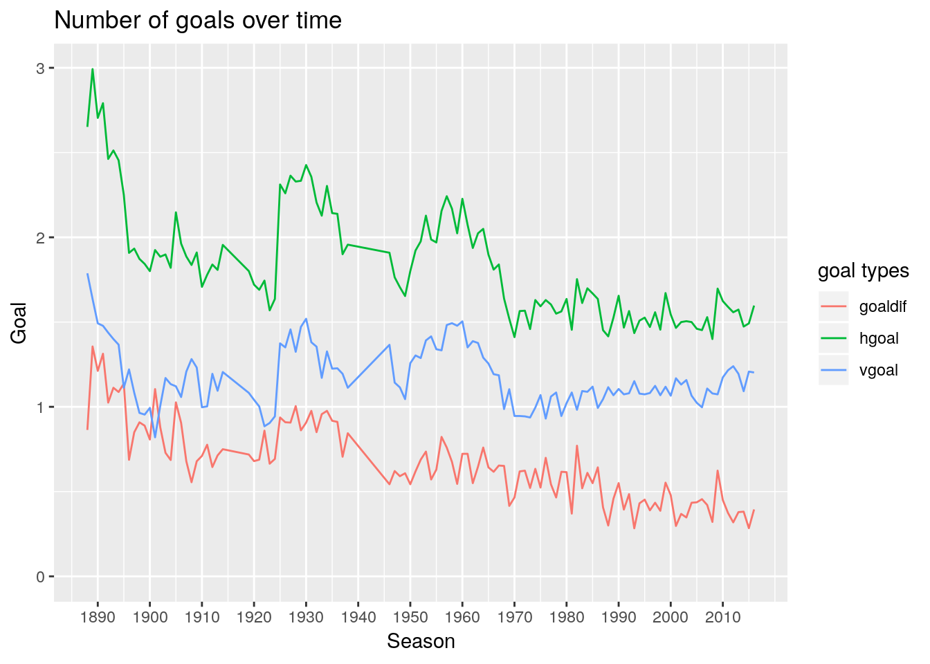

The tier 1 league was suspended for four seasons for WWI and seven for WWII, that’s why we see some straight lines during those years.

It is interesting to see goal difference has a clear trend of going down. Why does the home advantage decrease over the past 130 years? Hmm…

Which teams show up most in EPL?

## this is to lump the home teams into top five teams by appearance
topteams <- tier1 %>%  
  group_by(home) %>%
  mutate(num=n()) %>%
  ungroup() %>%
  mutate(topteams=fct_lump(home, 5)) %>%
  group_by(topteams, Season) %>%
  summarize(goaldif=mean(goaldif))

topteams %>%
  filter(topteams != "Other") %>%
  ggplot(aes(Season,goaldif, color=topteams))+
  geom_smooth() +
  geom_point() +
  expand_limits(y=0) +
  scale_x_continuous(breaks=seq(1890,2010,10)) +
      labs(x = "Season",
       y = "Goal differentials",
       title = "Goal differentials per match for the teams apprear most often")

## `geom_smooth()` using method = 'loess' and formula 'y ~ x'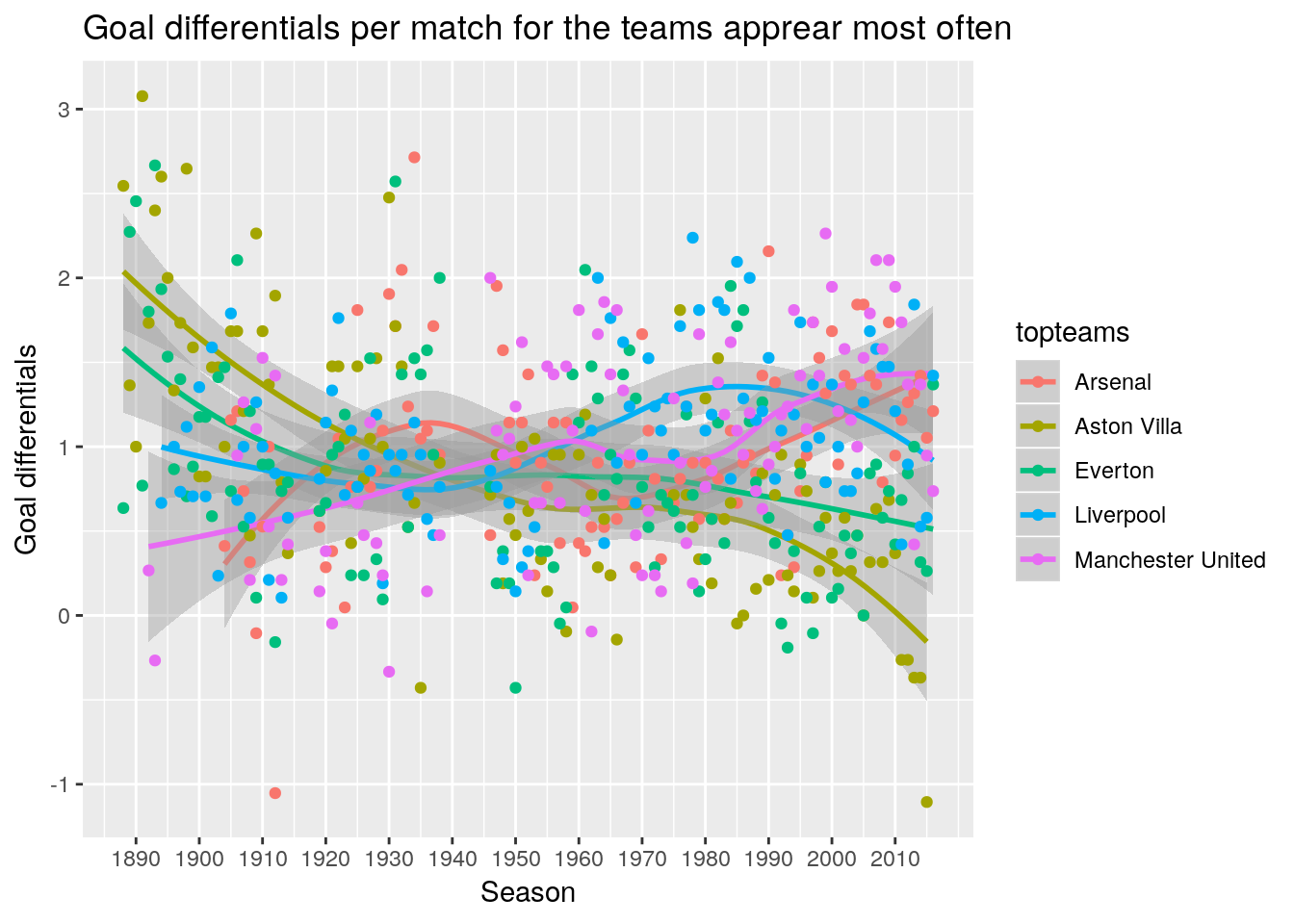

Now the question: do the championship teams win most of top 4 head-to-head? Does it happen that you lose to top contenders and still win the league?

tier1 %>%
  head()

##         Date Season            home          visitor  FT hgoal vgoal
## 1 1888-12-15   1888 Accrington F.C.      Aston Villa 1-1     1     1
## 2 1889-01-19   1888 Accrington F.C. Blackburn Rovers 0-2     0     2
## 3 1889-03-23   1888 Accrington F.C. Bolton Wanderers 2-3     2     3
## 4 1888-12-01   1888 Accrington F.C.          Burnley 5-1     5     1
## 5 1888-10-13   1888 Accrington F.C.     Derby County 6-2     6     2
## 6 1888-12-29   1888 Accrington F.C.          Everton 3-1     3     1
##   division tier totgoal goaldif result decade
## 1        1    1       2       0      D   1880
## 2        1    1       2      -2      A   1880
## 3        1    1       5      -1      A   1880
## 4        1    1       6       4      H   1880
## 5        1    1       8       4      H   1880
## 6        1    1       4       2      H   1880

# first calculate score for each season
# this is to make a long format for tier 1 data
tier1_gathered <- tier1 %>%
  select(Date, Season, home, visitor, hgoal, vgoal, result) %>%
  gather(key=homecourt, value=team, -Date, -Season, -hgoal, -vgoal, -result) 

## calculate rank for each season
ranked <- tier1_gathered %>%
  mutate(goal=ifelse(homecourt=="home", hgoal, vgoal)) %>% 
  mutate(ogoal=ifelse(homecourt=="home", vgoal, hgoal)) %>% 
  select(-hgoal, -vgoal) %>% 
  mutate(points=case_when(
    goal>ogoal ~ 3,
    goal<ogoal ~ 0,
    goal==ogoal ~ 1
    )) %>% 
  arrange(Date) %>%
  group_by(team, Season) %>%
  arrange(Date) %>%
  mutate(points_total=cumsum(points),  goaldiff=goal-ogoal, points_season=sum(points)) %>%  
  group_by(Season, team) %>% 
  summarise(points_season=sum(points), goal_season=sum(goal), ogoal_season=sum(ogoal), num_matches=n()) %>% 
  mutate(goal_diff=goal_season-ogoal_season) %>%
  group_by(Season) %>%
  arrange(Season, -points_season, -goal_diff) %>%
  mutate(rank=rank(desc(points_season),ties.method = 'first')) %>% 
  ungroup() 

How does the champions’ goal difference per game change over time, and points per game?

champions <- ranked %>%
  filter(rank==1) %>%
  group_by(Season) %>%
  mutate(points_match=points_season/num_matches, goal_diff_match=goal_diff/num_matches)

champions %>%
  ggplot(aes(Season,goal_diff_match)) +
  geom_point() +
  expand_limits(y=0)+
  geom_smooth() +
  scale_x_continuous(breaks=seq(1890,2010,10)) +
      labs(x = "Season",
       y = "Point differentials",
       title = "Point differentials per match for the champions")

## `geom_smooth()` using method = 'loess' and formula 'y ~ x'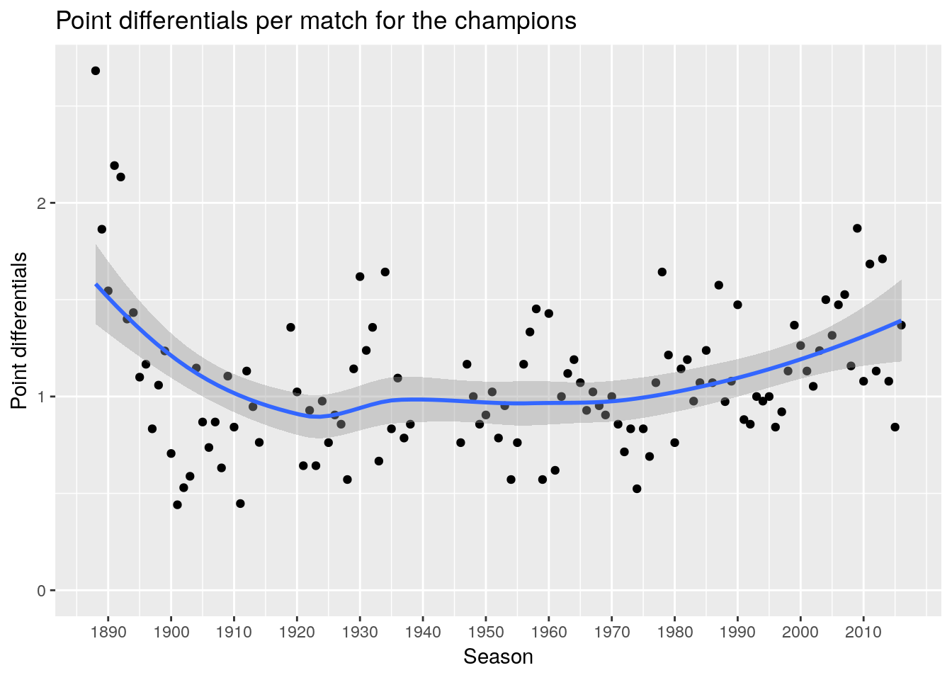

champions %>%
  ggplot(aes(Season,points_match)) +
  geom_point() +
  expand_limits(y=0)+
  geom_smooth() +
  scale_x_continuous(breaks=seq(1890,2010,10)) +
      labs(x = "Season",
       y = "Points per match",
       title = "Points per match for the champions")

## `geom_smooth()` using method = 'loess' and formula 'y ~ x'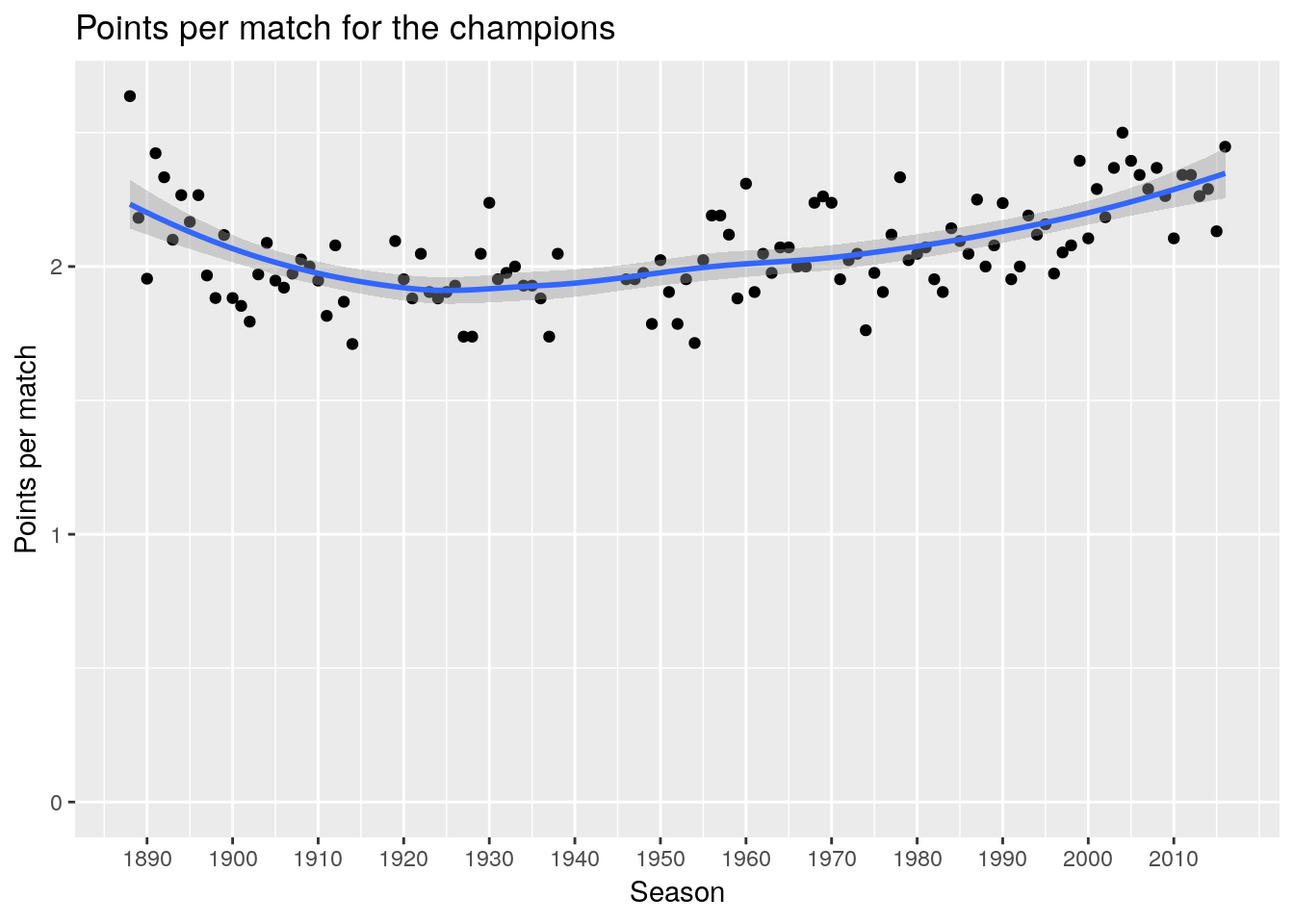

For the champions, we see the trend of points per game and goal difference per game is actually going up after 1920’s, opposite to the trend for average numbers across all teams each season. It seems the best teams are getting more dominating. An obvious explanation is the wealth concentration on the largest clubs.

How about other teams?

ranked %>%
  filter(rank<5) %>%
    ggplot(aes(Season,goal_diff, color=as.factor(rank)))+
  geom_smooth() +
  geom_point() +
  expand_limits(y=0) +
  scale_x_continuous(breaks=seq(1890,2010,10)) +
       labs(x = "Season",
       y = "Goal differentials per season",
       title = "Goal differentials for the top teams", 
       color = "ranking")

## `geom_smooth()` using method = 'loess' and formula 'y ~ x'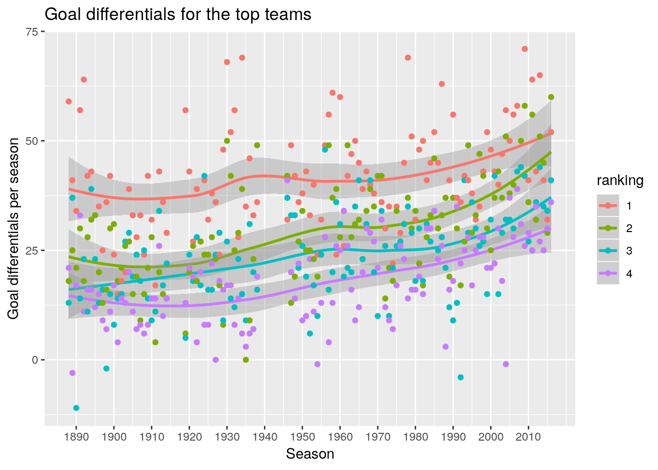

ranked %>%
  filter(rank>18) %>%
  ggplot(aes(Season,goal_diff, color=as.factor(rank)))+
  geom_smooth() +
  geom_point() +
  expand_limits(y=0) +
  scale_x_continuous(breaks=seq(1890,2010,10)) +
      labs(x = "Season",
       y = "Goal differentials per season",
       title = "Goal differentials for the worst teams", 
       color = "ranking")

## `geom_smooth()` using method = 'loess' and formula 'y ~ x'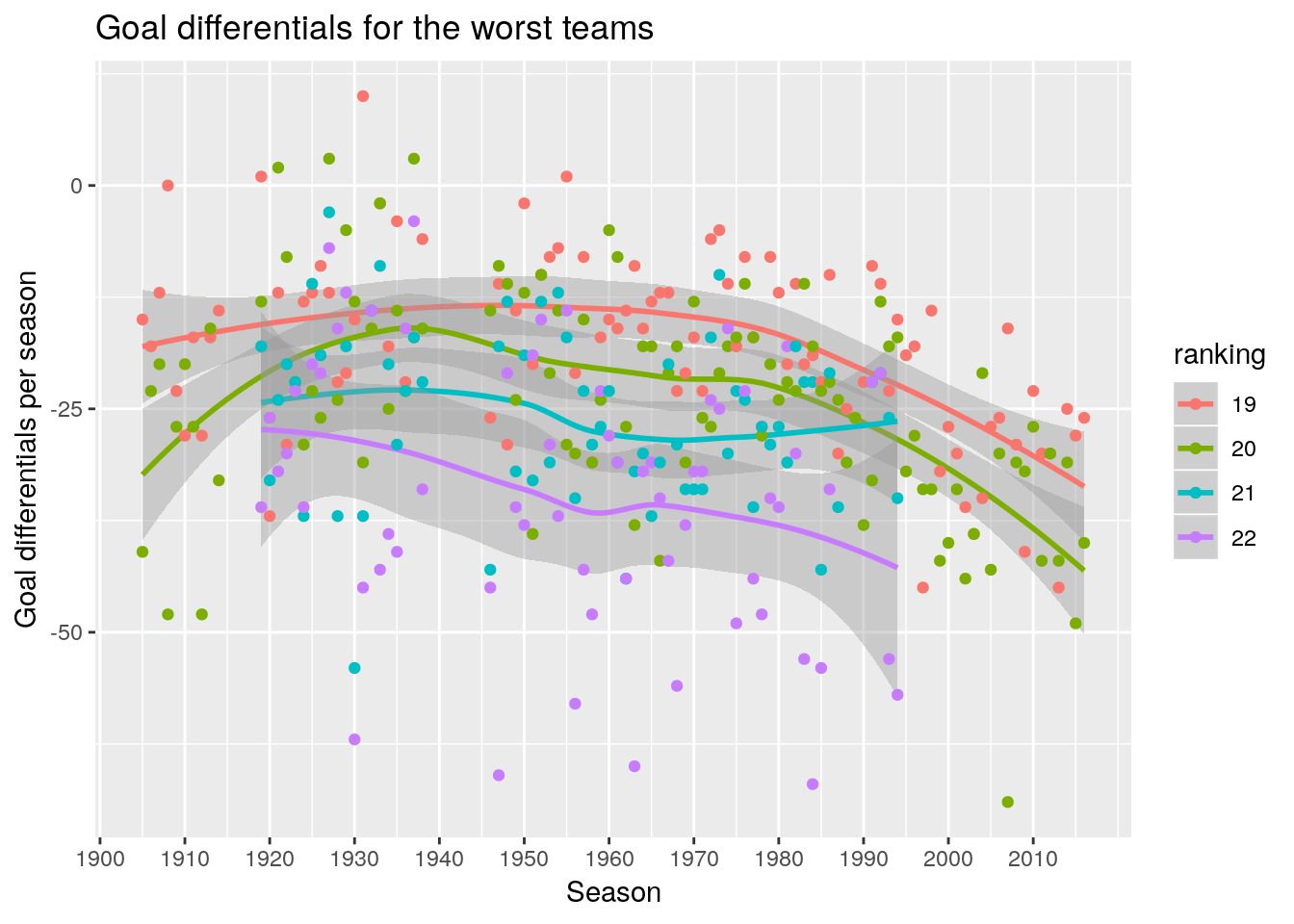

We see top 4 teams are all getting more dominating. The bottom ones (lower than 18) are getting worse. The number of teams have changed over the years, from 1992, the number of team is 20 in the EPL.

Now we turn to the question: what’s the points per match for the champions against top 4 (the other top 3, actually), vs against other teams? Are there situations they actually win more often against their title contenders?

team_rank <- ranked %>%
  select(Season, team, rank)

tier1_merge <- tier1 %>%
  left_join(team_rank, by=c("Season"="Season", "home"="team")) %>%
  mutate(home_rank=rank) %>%
  select(-rank) %>%
  left_join(team_rank, by=c("Season"="Season", "visitor"="team")) %>%
  mutate(visitor_rank=rank) %>%
  select(-rank) %>%
  tbl_df()

tier1_gathered2 <- tier1_merge %>%
  select(Date, Season, home, visitor, hgoal, vgoal, result, home_rank, visitor_rank) %>%
  gather(key=homecourt, value=team, -Date, -Season, -hgoal, -vgoal, -result, -home_rank, -visitor_rank) 

## a data set with Season, team, match level, with opponents status.
ranked2 <- tier1_gathered2 %>%
  mutate(goal=ifelse(homecourt=="home", hgoal, vgoal)) %>% 
  mutate(ogoal=ifelse(homecourt=="home", vgoal, hgoal)) %>% 
  mutate(team_rank=ifelse(homecourt=="home", home_rank, visitor_rank)) %>% 
  mutate(oppo_rank=ifelse(homecourt=="home", visitor_rank, home_rank)) %>% 
  select(-hgoal, -vgoal, -home_rank, -visitor_rank) %>% 
  mutate(points=case_when(
    goal>ogoal ~ 3,
    goal<ogoal ~ 0,
    goal==ogoal ~ 1
    )) %>% 
  arrange(Date) %>%
  mutate(team_top4=team_rank<5, oppo_top4=oppo_rank<5, champ=team_rank==1) %>%
  group_by(Season, team, oppo_top4) %>%
  mutate(points_top4=sum(points)) %>%
  arrange(Season, team, oppo_top4)

champs_points <- ranked2 %>%
  filter(team_rank==1) %>%
  group_by(Season, team, oppo_top4) %>% 
  summarise(points_season=sum(points), goal_season=sum(goal), ogoal_season=sum(ogoal), num_matches=n(), points_top4_season=mean(points_top4)) %>% 
  mutate(points_top4_match=points_top4_season/num_matches) 

champs_points %>%
  ggplot(aes(Season,points_top4_match, color=as.factor(oppo_top4)))+
  geom_smooth() +
  geom_point() +
  expand_limits(y=0) +
  scale_x_continuous(breaks=seq(1890,2010,10)) +
  geom_text(aes(label = team), vjust = 1, hjust = 1, check_overlap = TRUE, size=3) +
      labs(x = "Season",
       y = "Points per match",
       title = "Average points per game for the champions", 
       color = "Against top contenders")

## `geom_smooth()` using method = 'loess' and formula 'y ~ x'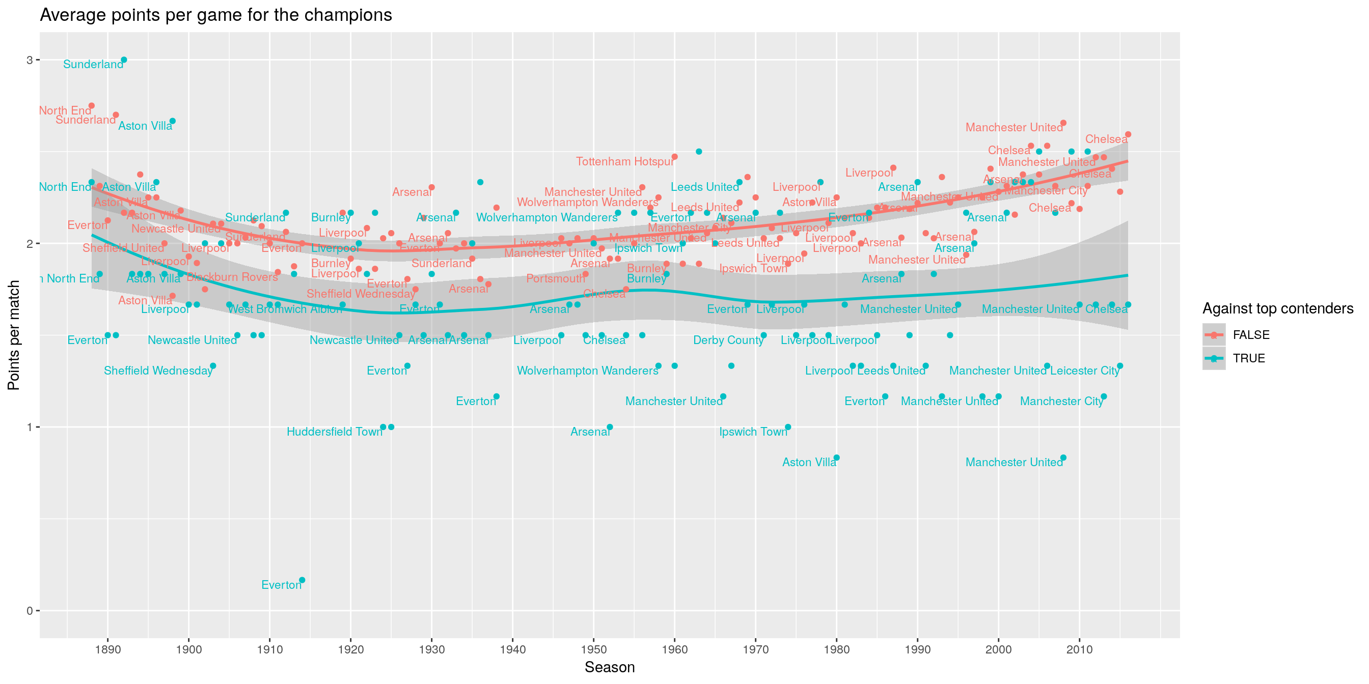

We see most cases points are higher if opponents are not top 4. But there are exceptions. Everton in 1919, Aston Villa in 1980 and Manchester United in 2008 have average points lower than 1, meaning on average they lose to the other top 3 opponents, but the winning percentage is much higher against other opponents.

Now we label those teams who have a higher winning percentage against other top 3 teams vs. lower ranked teams:

champs_points %>%
  arrange(Season, team, oppo_top4) %>%
  group_by(Season, team) %>%
  mutate(flag=points_top4_match>lag(points_top4_match)) %>%
  mutate(flag2=sum(flag, na.rm=TRUE)) %>%
  ggplot(aes(Season,points_top4_match, color=as.factor(flag2)))+
  geom_point() +
  expand_limits(y=0) +
  scale_x_continuous(breaks=seq(1890,2010,10)) +
  geom_text(aes(label = team), vjust = 1, hjust = 1, check_overlap = TRUE, size=3) +
    labs(x = "Season",
       y = "Points per match",
       title = "Average points per game for the champions", 
       color = "Score more against top contenders")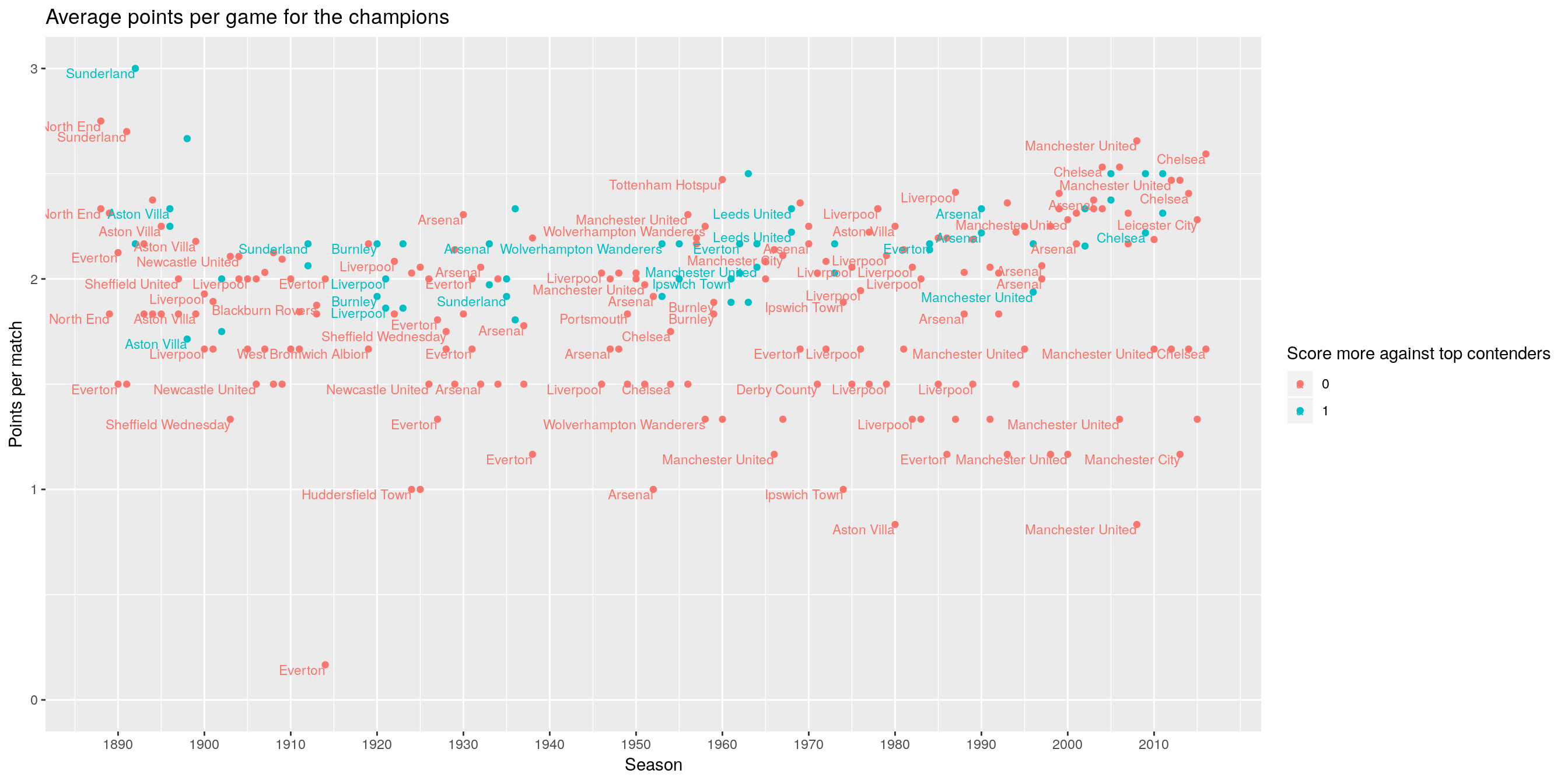 

There are not so many champions won more points from top contenders than other teams on average, but there are a few. Sunderland had won all games against top 4 contenders in 1892.

Overall, a team wins championship by winning bother situations. When they play against top contenders, at least they have 50% chance of winning. The expected score will be 4/3 if we consider equal chance of winning, losing, or tieing. Any champion below 4/3 against top contenders is under-performing. But acationally they won championships after losing to top contenders. Such as Mancheseter City in 2008.

Now let’s see how the toughness of a match impact the probability of winning.

library(lfe)

## Loading required package: Matrix

## 
## Attaching package: 'Matrix'

## The following object is masked from 'package:tidyr':
## 
##     expand

m1 <- felm(points ~ oppo_rank + oppo_top4 + homecourt | team | 0 | team, data=ranked2)
summary(m1)

## 
## Call:
##    felm(formula = points ~ oppo_rank + oppo_top4 + homecourt | team |      0 | team, data = ranked2) 
## 
## Residuals:
##     Min      1Q  Median      3Q     Max 
## -2.5332 -1.0030 -0.3324  1.1201  2.8685 
## 
## Coefficients:
##                   Estimate Cluster s.e. t value Pr(>|t|)    
## oppo_rank         0.040291     0.001037  38.844   <2e-16 ***
## oppo_top4TRUE    -0.130398     0.013466  -9.683   <2e-16 ***
## homecourtvisitor -0.804884     0.014822 -54.305   <2e-16 ***
## ---
## Signif. codes:  0 '***' 0.001 '**' 0.01 '*' 0.05 '.' 0.1 ' ' 1
## 
## Residual standard error: 1.217 on 95752 degrees of freedom
## Multiple R-squared(full model): 0.1506   Adjusted R-squared:  0.15 
## Multiple R-squared(proj model): 0.1408   Adjusted R-squared: 0.1402 
## F-statistic(full model, *iid*):253.3 on 67 and 95752 DF, p-value: < 2.2e-16 
## F-statistic(proj model):  3473 on 3 and 64 DF, p-value: < 2.2e-16

This is a fixed effect model on teams, with clustered standard error on teams. It shows opponent’s rank has a negative effect. If you are playing a team who is ranked 22, you are getting .4 point higher than if you play against a no. 12 team. Home court advantage is big: if you are playing at home, on average you are scoring .8 more points. If you are playing against top4, on average you score .13 less points.

I may think about how to see the champions progress: how many of them come from behind? How many getting better over time?