简介
在本文中我们用机器学习和统计的方法来分析红楼梦的作者。红楼梦是中国最著名的小说之一(https://en.wikipedia.org/wiki/Dream_of_the_Red_Chamber)。 大多数人认为前八十回为曹雪芹所作, 后四十回为后人续作。 除非我们从考古中发现证据,唯一能告诉我们的便是小说本身。我们可以从文章的用词风格来判断作者。 即使续作者尽量模仿原作者的风格,也很难不在字里行间露出自己固有的风格。(我们也许可以用同样的方法来鉴定真画和假画,但是需要有原作者的大量画作)。
我是从这里下载的红楼梦原著120回版(具体哪个版本我也没仔细研究): http://www.shuyaya.cc/book/2034/#download
我用了R中的 “Rwordseg” 来做中文分词。 就是把一句话分成词和词组。 然后用了 “cleanNLP” 得到分词频率矩阵 (“term frenquency matrix”)。 然后在最后一个模型用到 “topicmodels”。
读入文本进行分词
这一部分就是读入文本, 把它分为120回,每一回作为一个文本, 然后分词。
# analysis starts here
library(rticles)
library(cleanNLP)
library(readr)
library(stringi)
library(ggplot2)
library(glmnet)
library(ggrepel)
library(viridis)
library(magrittr)

library(topicmodels)
library(tidyverse)
library(rJava)
library(Rwordseg)
library(RColorBrewer)
library(tm)

require(readtext)
honglou1 <- readtext("~/projects/honglongmeng/honglou1.txt", text_field = "texts")

# here is to split into chapters using stringr's splitting functions
my_split <- function(text) {
    pattern <- '第.{1,3}回 '
    x <- str_split(text, pattern)[[1]]
    y <- str_extract_all(text, pattern)[[1]]
    data.frame(
        chapter = (1:length(x)) - 1,
        text = str_trim(x),
        header = c(y, "")
    )
}

chaps <- my_split(honglou1$text)


hong <- chaps %>%
    mutate(txt = as.character(text))

# use Rwordseg's segmentCN to get tokens from text.
honglou <- tbl_df(hong) %>%
     mutate(token=segmentCN(txt)) %>%
     mutate(id=chapter) %>%
     select(id, token)
第一种模型
生成分词以后, 我用“cleanNLP”里的一个函数叫“get_tfidf”来取得分词频率矩阵。
首先我想到的办法是把所有章节分为“training” 和“test”。 这是机器学习的常用办法。 在“training” 章节中, 如果是前八十章, 我标识作者为“Cao”,否则标识为“unknown”。
然后我用“elastic net” (combination of lasso and ridge) (一种机器学习方法)在training sample。 然后在test sample中来预测作者。
这样我们得到每一章作者是曹雪芹的概率。
# make it long format: from each row for each chapter to one row for each token.
hongloumeng <- honglou %>%
    group_by(id) %>%
    unnest(token) %>%
    filter(id>0) %>%
    ungroup()

# get length (how many tokens in each chapter) on the way for each chapter
hongloumeng %>%
  group_by(id) %>%
  summarize(sent_len = n()) %$%
  quantile(sent_len, seq(0,1,0.1))
## 0% 10% 20% 30% 40% 50% 60% 70% 80% 90%
## 594.0 3229.6 3591.4 3852.2 4154.2 4311.5 4570.4 4750.0 5055.0 5744.5
## 100%
## 7114.0# frequency of tokens; get the top ones
freq <- hongloumeng %>%
group_by(token) %>%
summarize(count = n()) %>%
top_n(n = 100, count) %>%
arrange(desc(count))
# set up the ususal format for text analysis
honglou2 <- hongloumeng %>%
mutate(sid=1, tid=1, lemma=NA, upos=NA, pos=NA, cid=NA, word=token)
# assign first 80 chapters to Cao and the last 40 to unknown.
chapters <- honglou2 %>%
group_by(id) %>%
summarise(chapter=mean(id)) %>%
mutate(author=ifelse(chapter<81, "cao", "unknown"))
# use cleanNLP's get_tfidf to get the term frequency matrix
# tfidf <- honglou2 %>%
# get_tfidf(type = "tfidf", tf_weight = "dnorm", token_var="word")
#honglou_pca <- tidy_pca(tfidf$tfidf, chapters)
#ggplot(honglou_pca, aes(PC1, PC2)) +
# geom_point(aes(color=chapter))
#mat.honglou <- get_tfidf(honglou2, min_df = 0.1, max_df = .9, type = "tf",
# tf_weight = "raw", doc_var = "id", token_var="word")
# a second specification for the term freqency matrix.
mat.honglou <- honglou2 %>%
get_tfidf(type = "tf", tf_weight = "dnorm", token_var="word")
## tf2 <- honglou2 %>%
## get_tfidf(min_df = 0, max_df = 1, type = "tf",
## tf_weight = "raw", token_var="word")
# random assign traing and testing samples
set.seed(1)
chapters <- chapters %>%
mutate(training = as.logical(rbinom(length(chapter), 1, .5))) %>%
mutate(y=as.numeric(author=="cao"))
chapters.train <- chapters %>% filter(training==1)
model <- cv.glmnet(mat.honglou$tf[chapters$training,], chapters.train$y,
family = "binomial", alpha=.9)
chapters$pred <- predict(model, newx=mat.honglou$tf, type='response', s=model$lambda.1se)
## ggplot(chapters, aes(chapter, pred)) +
## geom_boxplot(aes(fill = author))
ggplot(chapters, aes(x = chapter, y = pred, color = training)) +geom_point() +geom_vline(xintercept=80) +geom_vline(xintercept=108) + geom_text(aes(chapter-3,pred, label = chapter), data = chapters %>% filter((pred<.85 & chapter<81 & training==0) | (pred > .5 & chapter>80 & training==0)))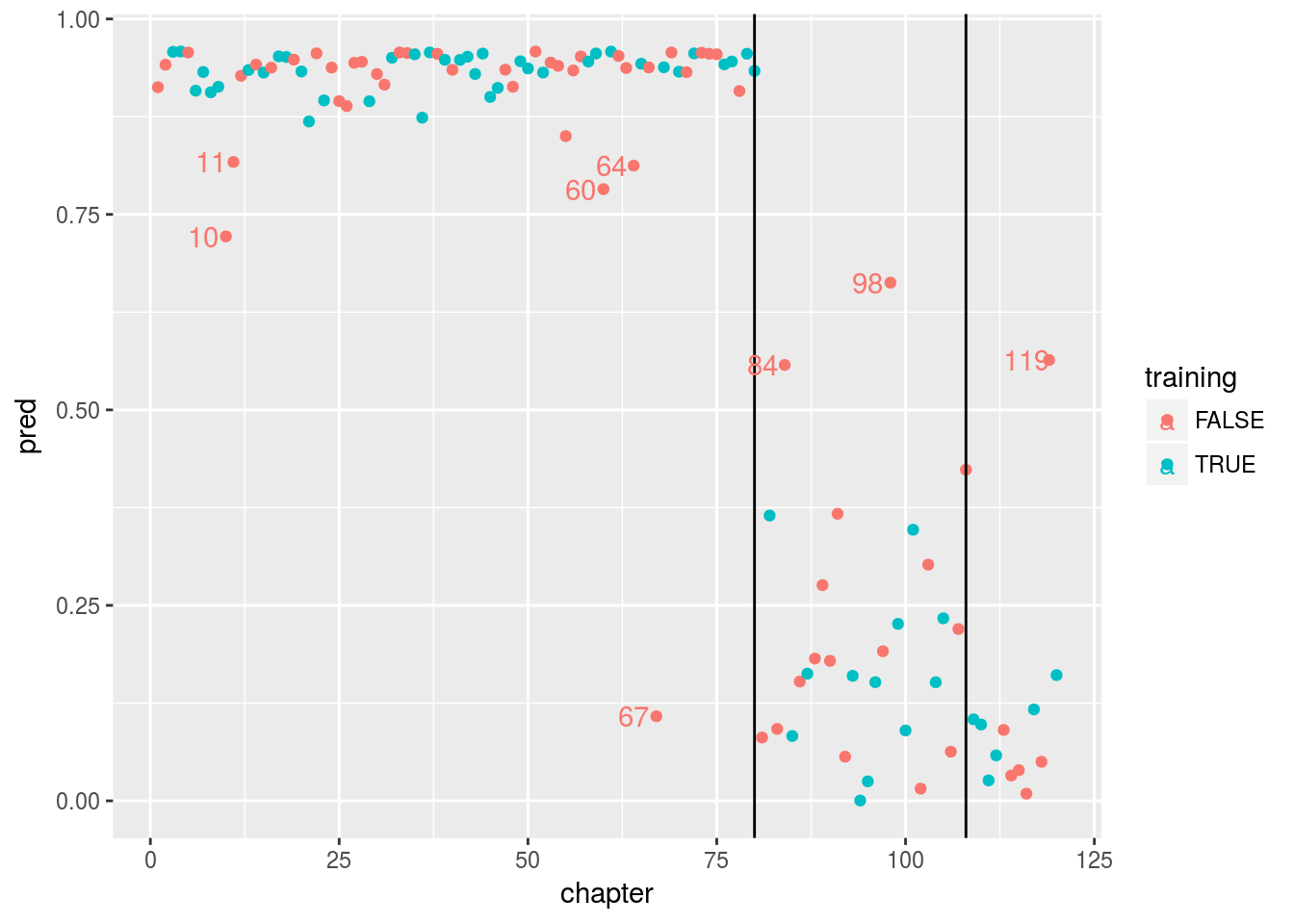
在图中,我画了两条竖线,80和108回。有些人认为曹的原作只有108回。
两种不同颜色代表training or test。 我们看到如果说前80回作者是“Cao”,那么后40回作者不大可能是“Cao”。 甚至前80回中有几回也与其他章用词不太一致,例如10, 11, 60, 64, 67。 特别是67, 不太可能作者是“Cao”。 在后40回中, 84,98,119 则与前80回风格较为一致。
第二种模型
第二种模型是某种程度上的改善。 在第一种模型中,我们把前80回标为“Cao”,后40回为“unknown”。我们没有引入不确定性。 这里,我们假设后40回有百分之二十可能作者是“Cao”。这样我们引入不确定性。 我们还是用同一种统计模型elastic net。
# here we introduce uncertainty: suppose the last 40 chapters have 20% chance been written by Cao.

set.seed(1)
chapters.matrix <- matrix(NA,120,100)
training.matrix <- matrix(NA, 120, 100)
for (i in (1:100)){

chapters2 <- honglou2 %>%
    group_by(id) %>%
    summarise(chapter=mean(id)) %>%
    mutate(author=ifelse(chapter<81, "cao", ifelse(rbinom(40,1,.2),"cao","unknown"))) %>%
    mutate(training = as.logical(rbinom(length(chapter), 1, .5))) %>%
    mutate(y=as.numeric(author=="cao"))

chapters2.train <- chapters2 %>% filter(training==1)
model2 <- cv.glmnet(mat.honglou$tf[chapters2$training,], chapters2.train$y,
                   family = "binomial", alpha=.9)

chapters2$pred <- predict(model2, newx=mat.honglou$tf, type='response', s=model2$lambda.1se)

chapters.matrix[, i] <- chapters2$pred
training.matrix[,i] <- chapters2$training

}
## ggplot(chapters, aes(chapter, pred)) +
##   geom_boxplot(aes(fill = author))

wide <- bind_cols(data.frame(chapter=1:120), as.data.frame(chapters.matrix))
wide2 <- bind_cols(data.frame(chapter=1:120), as.data.frame(training.matrix))
long <- wide %>% gather("sim", "yhat",2:101)
long <- long %>% mutate(sim = as.integer(sub("V", "", sim)))
long2 <- wide2 %>% gather("sim", "training",2:101)
long2 <- long2 %>% mutate(sim = as.integer(sub("V", "", sim)))
long3 <- bind_cols(long, long2)[,c(1:3, 6)]

merged <- long3 %>% left_join(chapters2 %>% select(-training), by = "chapter")

#ggplot(merged, aes(y = yhat, x = chapter, group = chapter)) + geom_boxplot()
ggplot(merged, aes(y = yhat, x = chapter, group = chapter)) +
  geom_boxplot() + facet_grid(training ~ .)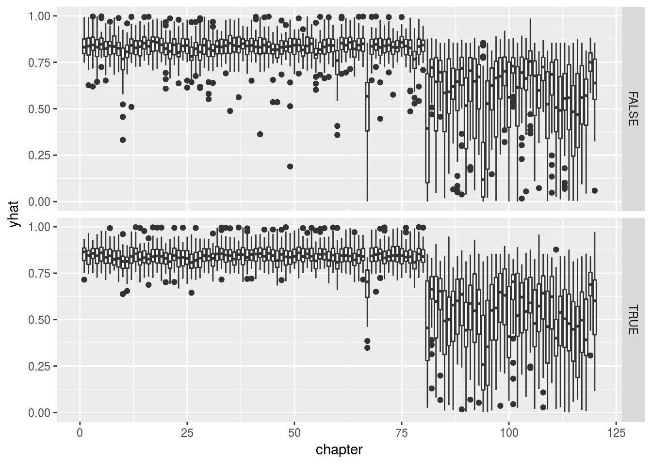
在这里我画的是重复100次取样后的box plot, 上面是testing, 下面是training。 第二种模型和第一种结论类似,只是引入不确定性。
第三种模型
前两次的模型有个显然的假设,就是我们假设前80回是同一个作者,然后我们来判断是否后40回是否属于同一作者。也就是说这里我们只能根据前80回为同一作者来推断后40回的作者。 如果前80回不是一个作者那么我们的推断就不成立。
我想到也许应该用一种更好的模型, 就是每一章都有一定的概率属于“Cao”。 然后我们来估计这些概率。我发现这属于“topic models”。
“topic models” 是用来研究文本中有几个主题的,但是我们没有理由不能把它用于研究作者。因为归根结底主题就是词汇组合,而作者也可视为词汇组合。
现在我们唯一的假设是有两个作者, 严格说,是有两个“主题”,或者说,这120回可以分为两组,至于两组为什么不同,我姑且认为是作者不同,因为我们是从用词频率分析的。 也可以假设有三个作者来分析,等等,分析方法都一样。
这里我们用LDA(Linear Dirichlet Allocation) 分析每一章属于“Cao” 的概率。
set.seed(1)

mat.honglou2 <- honglou2 %>%
    get_tfidf(type = "tf", tf_weight = "raw", token_var="word",
    min_df=.05, max_df=.95)
colnames(mat.honglou2$tf) <- mat.honglou2$vocab
lda2 <- LDA(mat.honglou2$tf, k = 2, method="Gibbs", control = list(seed = 1, burnin = 1000, thin = 100, iter = 1000))

plot(topics(lda2))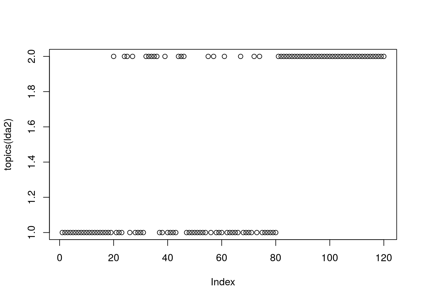
lda_topics <- as.data.frame(posterior(lda2)$topics)
names(lda_topics) <- c('prob1', 'prob2')

newdata <- bind_cols(chapters, lda_topics)
topics <- posterior(lda2)[["topics"]]
#heatmap(topics, scale = "none")

ggplot(newdata, aes(y = prob1, x = chapter, group = chapter)) +
 geom_point() +geom_vline(xintercept=80) +geom_vline(xintercept=108) + geom_text(aes(chapter-3,prob1, label = chapter), data = newdata %>% filter((prob1<.5 & chapter<81 ) | (prob1 > .5 & chapter>80 )))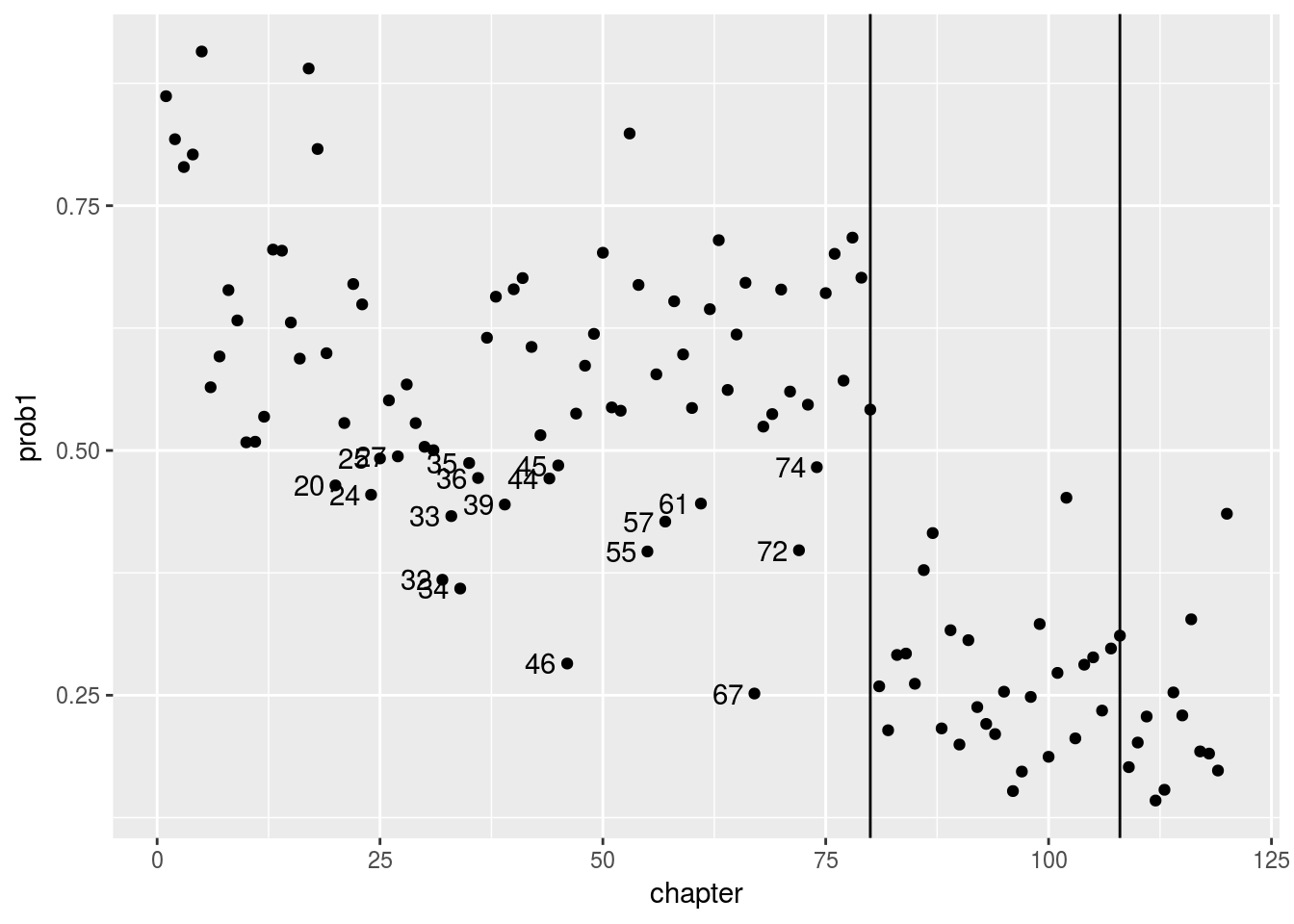
我们看到前80回有19回是作者1写的概率低于50%。 尤其第67回, 只有25%的概率是作者1写的。 在后40回中, 没有一回概率大于50%! 作者1应该是曹雪芹。这里我们不能分析出作者是谁,只是说后40回的作者与前80回大多数章节的作者不同。
下面我们看看作者1,2最常用的前50个词, 严格说是从LDA模型中的posterior得到的主题1,2最常出现的50个词。
terms1 <- posterior(lda2)$terms[1,]
terms2 <- posterior(lda2)$terms[2,]
head(sort(terms1, decreasing=TRUE), 50)
## 吃 贾母 至 众人 方 贾
## 0.010980743 0.006512404 0.005828384 0.005401982 0.005401982 0.005330915
## 凤 珍 一面 黛玉 字 酒
## 0.004593594 0.004167192 0.004007291 0.003971758 0.003794090 0.003660840
## 此 两个 花 如此 茶 皆
## 0.003625306 0.003536472 0.003367688 0.003341038 0.003296621 0.003190021
## 大家 他们 竟 亦 尤氏 晴雯
## 0.003074537 0.003047887 0.003039003 0.003030120 0.002994586 0.002914636
## 向 使 日 未 如 湘云
## 0.002896869 0.002887986 0.002852452 0.002834686 0.002754735 0.002754735
## 比 不过 老 听说 忽 三
## 0.002674785 0.002621485 0.002612601 0.002577068 0.002568184 0.002541534
## 薛蟠 其 或 香 所 毕
## 0.002523767 0.002514884 0.002506001 0.002497117 0.002488234 0.002488234
## 生 让 并 只见 后 原来
## 0.002479351 0.002470467 0.002443817 0.002399400 0.002319450 0.002310566
## 岂 而
## 0.002301683 0.002301683head(sort(terms2, decreasing=TRUE), 50)## 袭人 凤姐 姑娘 王夫人 宝钗 给
## 0.009255081 0.009173040 0.008836671 0.008730017 0.008286994 0.007753725
## 老太太 贾母 丫头 太太 贾琏 你们
## 0.007745521 0.007245069 0.006744617 0.006695392 0.006252369 0.006194940
## 奶奶 贾政 死 平儿 老爷 听见
## 0.006030857 0.005792938 0.005472976 0.005341710 0.005095586 0.005054566
## 黛玉 告诉 东西 他们 回来 爷
## 0.005038157 0.004865871 0.004562318 0.004307990 0.004307990 0.004225948
## 进来 病 哭 做 薛姨妈 只见
## 0.004193132 0.003963416 0.003897783 0.003782925 0.003717292 0.003586026
## 瞧 紫鹃 鸳鸯 过来 这个 这样
## 0.003577822 0.003405535 0.003405535 0.003356310 0.003339902 0.003274269
## 找 咱们 心里 闹 这些 一面
## 0.003266065 0.003159411 0.003118391 0.003077370 0.003044553 0.003028145
## 跟 却 两个 林 这么 姐姐
## 0.003019941 0.002987124 0.002831246 0.002782021 0.002749205 0.002699980
## 所以 出去
## 0.002699980 0.002683572